Artificial neural network

Part of a series on
Machine learning and data mining
show Problems Classification Clustering Regression Anomaly detection Data Cleaning AutoML Association rules Reinforcement learning Structured prediction Feature engineering Feature learning Online learning Semi-supervised learning Unsupervised learning Learning to rank Grammar induction
show Supervised learning (classification • regression) Decision trees Ensembles Bagging Boosting Random forest k-NN Linear regression Naive Bayes Artificial neural networks Logistic regression Perceptron Relevance vector machine (RVM) Support vector machine (SVM)
show Clustering BIRCH CURE Hierarchical k-means Expectation–maximization (EM) DBSCAN OPTICS Mean shift
show Dimensionality reduction Factor analysis CCA ICA LDA NMF PCA PGD t-SNE
show Structured prediction Graphical models Bayes net Conditional random field Hidden Markov
show Anomaly detection k-NN Local outlier factor
hide Artificial neural network Autoencoder Cognitive computing Deep learning DeepDream Multilayer perceptron RNN LSTM GRU ESN Restricted Boltzmann machine GAN SOM Convolutional neural network U-Net Transformer Spiking neural network Memtransistor Electrochemical RAM (ECRAM)
show Reinforcement learning Q-learning SARSA Temporal difference (TD)
show Theory Bias–variance tradeoff Computational learning theory Empirical risk minimization Occam learning PAC learning Statistical learning VC theory
show Machine-learning venues NeurIPS ICML ML JMLR ArXiv:cs.LG
show Related articles Glossary of artificial intelligence List of datasets for machine-learning research Outline of machine learning
v t

Part of a series on
Artificial intelligence
hide Major goals Artificial general intelligence Planning Computer vision General game playing Knowledge reasoning Machine learning Natural language processing Robotics
hide Approaches Symbolic Deep learning Bayesian networks Evolutionary algorithms
hide Philosophy Ethics Existential risk Turing test Chinese room Control problem Friendly AI
hide History Timeline Progress AI winter
hide Technology Applications Projects Programming languages
hide Glossary Glossary
v t

Complex systems
Topics
show Self-organization Emergence
show Collective behavior Social dynamics Collective intelligence Collective action Self-organized criticality Herd mentality Phase transition Agent-based modelling Synchronization Ant colony optimization Particle swarm optimization Swarm behaviour Collective consciousness
show Networks Scale-free networks Social network analysis Small-world networks Centrality Motifs Graph theory Scaling Robustness Systems biology Dynamic networks Adaptive networks
show Evolution and adaptation Artificial neural network Evolutionary computation Genetic algorithms Genetic programming Artificial life Machine learning Evolutionary developmental biology Artificial intelligence Evolutionary robotics Evolvability
show Pattern formation Fractals Reaction–diffusion systems Partial differential equations Dissipative structures Percolation Cellular automata Spatial ecology Self-replication Geomorphology
show Systems theory and Cybernetics Autopoiesis Information theory Entropy Feedback Goal-oriented Homeostasis Operationalization Second-order cybernetics Self-reference System dynamics Systems science Sensemaking Variety Theory of computation
show Nonlinear dynamics Time series analysis Ordinary differential equations Phase space Attractors Population dynamics Chaos Multistability Bifurcation Coupled map lattices
show Game theory Prisoner's dilemma Rational choice theory Bounded rationality Evolutionary game theory
v t

Network science
Theory
Graph Complex network Contagion Small-world Scale-free Community structure Percolation Evolution Controllability Graph drawing Social capital Link analysis Optimization Reciprocity Closure Homophily Transitivity Preferential attachment Balance theory Network effect Social influence
Network types
Informational (computing) Telecommunication Transport Social Scientific collaboration Biological Artificial neural Interdependent Semantic Spatial Dependency Flow on-Chip
Graphs
Features Clique Component Cut Cycle Data structure Edge Loop Neighborhood Path Vertex Adjacency list / matrix Incidence list / matrix Types Bipartite Complete Directed Hyper Multi Random Weighted
Metrics Algorithms
Centrality Degree Motif Clustering Degree distribution Assortativity Distance Modularity Efficiency
Models
Topology Random graph Erdős–Rényi Barabási–Albert Fitness model Watts–Strogatz Exponential random (ERGM) Random geometric (RGG) Hyperbolic (HGN) Hierarchical Stochastic block Blockmodeling Maximum entropy Soft configuration LFR Benchmark Dynamics Boolean network agent based Epidemic/SIR
Lists Categories
Topics Software Network scientists Category:Network theory Category:Graph theory
v t

An artificial neural network is an interconnected group of nodes, inspired by a simplification of neurons in a brain. Here, each circular node represents an artificial neuron and an arrow represents a connection from the output of one artificial neuron to the input of another.

Artificial neural networks (ANNs), usually simply called neural networks (NNs), are computing systems inspired by the biological neural networks that constitute animal brains.

An ANN is based on a collection of connected units or nodes called artificial neurons, which loosely model the neurons in a biological brain. Each connection, like the synapses in a biological brain, can transmit a signal to other neurons. An artificial neuron receives a signal then processes it and can signal neurons connected to it. The "signal" at a connection is a real number, and the output of each neuron is computed by some non-linear function of the sum of its inputs. The connections are called edges. Neurons and edges typically have a weight that adjusts as learning proceeds. The weight increases or decreases the strength of the signal at a connection. Neurons may have a threshold such that a signal is sent only if the aggregate signal crosses that threshold. Typically, neurons are aggregated into layers. Different layers may perform different transformations on their inputs. Signals travel from the first layer (the input layer), to the last layer (the output layer), possibly after traversing the layers multiple times.

Training[]

Neural networks learn (or are trained) by processing examples, each of which contains a known "input" and "result," forming probability-weighted associations between the two, which are stored within the data structure of the net itself. The training of a neural network from a given example is usually conducted by determining the difference between the processed output of the network (often a prediction) and a target output. This difference is the error. The network then adjusts its weighted associations according to a learning rule and using this error value. Successive adjustments will cause the neural network to produce output which is increasingly similar to the target output. After a sufficient number of these adjustments the training can be terminated based upon certain criteria. This is known as supervised learning.

Such systems "learn" to perform tasks by considering examples, generally without being programmed with task-specific rules. For example, in image recognition, they might learn to identify images that contain cats by analyzing example images that have been manually labeled as "cat" or "no cat" and using the results to identify cats in other images. They do this without any prior knowledge of cats, for example, that they have fur, tails, whiskers, and cat-like faces. Instead, they automatically generate identifying characteristics from the examples that they process.

History[]

Warren McCulloch and Walter Pitts^[1] (1943) opened the subject by creating a computational model for neural networks.^[2] In the late 1940s, D. O. Hebb^[3] created a learning hypothesis based on the mechanism of neural plasticity that became known as Hebbian learning. Farley and Wesley A. Clark^[4] (1954) first used computational machines, then called "calculators", to simulate a Hebbian network. Rosenblatt^[5] (1958) created the perceptron.^[6] The first functional networks with many layers were published by Ivakhnenko and Lapa in 1965, as the Group Method of Data Handling.^[7][8][9] The basics of continuous backpropagation^{[7][10][11][12]} were derived in the context of control theory by Kelley^[13] in 1960 and by Bryson in 1961,^[14] using principles of dynamic programming. Thereafter research stagnated following Minsky and Papert (1969),^[15] who discovered that basic perceptrons were incapable of processing the exclusive-or circuit and that computers lacked sufficient power to process useful neural networks.

In 1970, Seppo Linnainmaa published the general method for automatic differentiation (AD) of discrete connected networks of nested differentiable functions.^[16][17] In 1973, Dreyfus used backpropagation to adapt parameters of controllers in proportion to error gradients.^[18] Werbos's (1975) backpropagation algorithm enabled practical training of multi-layer networks. In 1982, he applied Linnainmaa's AD method to neural networks in the way that became widely used.^[10][19]

The development of metal–oxide–semiconductor (MOS) very-large-scale integration (VLSI), in the form of complementary MOS (CMOS) technology, enabled increasing MOS transistor counts in digital electronics. This provided more processing power for the development of practical artificial neural networks in the 1980s.^[20]

In 1986 Rumelhart, Hinton and Williams showed that backpropagation learned interesting internal representations of words as feature vectors when trained to predict the next word in a sequence.^[21]

In 1992, max-pooling was introduced to help with least-shift invariance and tolerance to deformation to aid 3D object recognition.^[22][23][24] Schmidhuber adopted a multi-level hierarchy of networks (1992) pre-trained one level at a time by unsupervised learning and fine-tuned by backpropagation.^[25]

Geoffrey Hinton et al. (2006) proposed learning a high-level representation using successive layers of binary or real-valued latent variables with a restricted Boltzmann machine^[26] to model each layer. In 2012, Ng and Dean created a network that learned to recognize higher-level concepts, such as cats, only from watching unlabeled images.^[27] Unsupervised pre-training and increased computing power from GPUs and distributed computing allowed the use of larger networks, particularly in image and visual recognition problems, which became known as "deep learning".^[28]

Ciresan and colleagues (2010)^[29] showed that despite the vanishing gradient problem, GPUs make backpropagation feasible for many-layered feedforward neural networks.^[30] Between 2009 and 2012, ANNs began winning prizes in ANN contests, approaching human level performance on various tasks, initially in pattern recognition and machine learning.^[31][32] For example, the bi-directional and multi-dimensional long short-term memory (LSTM)^{[33][34][35][36]} of Graves et al. won three competitions in connected handwriting recognition in 2009 without any prior knowledge about the three languages to be learned.^[35][34]

Ciresan and colleagues built the first pattern recognizers to achieve human-competitive/superhuman performance^[37] on benchmarks such as traffic sign recognition (IJCNN 2012).

Models[]

This section may be confusing or unclear to readers. Please help clarify the section. There might be a discussion about this on the talk page. (April 2017) (Learn how and when to remove this template message)

Neuron and myelinated axon, with signal flow from inputs at dendrites to outputs at axon terminals

ANNs began as an attempt to exploit the architecture of the human brain to perform tasks that conventional algorithms had little success with. They soon reoriented towards improving empirical results, mostly abandoning attempts to remain true to their biological precursors. Neurons are connected to each other in various patterns, to allow the output of some neurons to become the input of others. The network forms a directed, weighted graph.^[38]

An artificial neural network consists of a collection of simulated neurons. Each neuron is a node which is connected to other nodes via links that correspond to biological axon-synapse-dendrite connections. Each link has a weight, which determines the strength of one node's influence on another.^[39]

Components of ANNs[]

Neurons[]

ANNs are composed of artificial neurons which are conceptually derived from biological neurons. Each artificial neuron has inputs and produces a single output which can be sent to multiple other neurons. The inputs can be the feature values of a sample of external data, such as images or documents, or they can be the outputs of other neurons. The outputs of the final output neurons of the neural net accomplish the task, such as recognizing an object in an image.

To find the output of the neuron, first we take the weighted sum of all the inputs, weighted by the weights of the connections from the inputs to the neuron. We add a bias term to this sum. This weighted sum is sometimes called the activation. This weighted sum is then passed through a (usually nonlinear) activation function to produce the output. The initial inputs are external data, such as images and documents. The ultimate outputs accomplish the task, such as recognizing an object in an image.^[40]

Connections and weights[]

The network consists of connections, each connection providing the output of one neuron as an input to another neuron. Each connection is assigned a weight that represents its relative importance.^[38] A given neuron can have multiple input and output connections.^[41]

Propagation function[]

The propagation function computes the input to a neuron from the outputs of its predecessor neurons and their connections as a weighted sum.^[38] A bias term can be added to the result of the propagation.^[42]

Organization[]

The neurons are typically organized into multiple layers, especially in deep learning. Neurons of one layer connect only to neurons of the immediately preceding and immediately following layers. The layer that receives external data is the input layer. The layer that produces the ultimate result is the output layer. In between them are zero or more hidden layers. Single layer and unlayered networks are also used. Between two layers, multiple connection patterns are possible. They can be fully connected, with every neuron in one layer connecting to every neuron in the next layer. They can be pooling, where a group of neurons in one layer connect to a single neuron in the next layer, thereby reducing the number of neurons in that layer.^[43] Neurons with only such connections form a directed acyclic graph and are known as feedforward networks.^[44] Alternatively, networks that allow connections between neurons in the same or previous layers are known as recurrent networks.^[45]

Hyperparameter[]

A hyperparameter is a constant parameter whose value is set before the learning process begins. The values of parameters are derived via learning. Examples of hyperparameters include learning rate, the number of hidden layers and batch size.^[46] The values of some hyperparameters can be dependent on those of other hyperparameters. For example, the size of some layers can depend on the overall number of layers.

Learning[]

This section includes a list of references, related reading or external links, but its sources remain unclear because it lacks inline citations. Please help to improve this section by introducing more precise citations. (August 2019) (Learn how and when to remove this template message)

Learning is the adaptation of the network to better handle a task by considering sample observations. Learning involves adjusting the weights (and optional thresholds) of the network to improve the accuracy of the result. This is done by minimizing the observed errors. Learning is complete when examining additional observations does not usefully reduce the error rate. Even after learning, the error rate typically does not reach 0. If after learning, the error rate is too high, the network typically must be redesigned. Practically this is done by defining a cost function that is evaluated periodically during learning. As long as its output continues to decline, learning continues. The cost is frequently defined as a statistic whose value can only be approximated. The outputs are actually numbers, so when the error is low, the difference between the output (almost certainly a cat) and the correct answer (cat) is small. Learning attempts to reduce the total of the differences across the observations.^[38] Most learning models can be viewed as a straightforward application of optimization theory and statistical estimation.

Learning rate[]

The learning rate defines the size of the corrective steps that the model takes to adjust for errors in each observation. A high learning rate shortens the training time, but with lower ultimate accuracy, while a lower learning rate takes longer, but with the potential for greater accuracy. Optimizations such as Quickprop are primarily aimed at speeding up error minimization, while other improvements mainly try to increase reliability. In order to avoid oscillation inside the network such as alternating connection weights, and to improve the rate of convergence, refinements use an adaptive learning rate that increases or decreases as appropriate.^[47] The concept of momentum allows the balance between the gradient and the previous change to be weighted such that the weight adjustment depends to some degree on the previous change. A momentum close to 0 emphasizes the gradient, while a value close to 1 emphasizes the last change.

Cost function[]

While it is possible to define a cost function ad hoc, frequently the choice is determined by the function's desirable properties (such as convexity) or because it arises from the model (e.g. in a probabilistic model the model's posterior probability can be used as an inverse cost).

Backpropagation[]

Backpropagation is a method used to adjust the connection weights to compensate for each error found during learning. The error amount is effectively divided among the connections. Technically, backprop calculates the gradient (the derivative) of the cost function associated with a given state with respect to the weights. The weight updates can be done via stochastic gradient descent or other methods, such as Extreme Learning Machines,^[48] "No-prop" networks,^[49] training without backtracking,^[50] "weightless" networks,^[51][52] and non-connectionist neural networks.

Learning paradigms[]

This section includes a list of references, related reading or external links, but its sources remain unclear because it lacks inline citations. Please help to improve this section by introducing more precise citations. (August 2019) (Learn how and when to remove this template message)

The three major learning paradigms are supervised learning, unsupervised learning and reinforcement learning. They each correspond to a particular learning task

Supervised learning[]

Supervised learning uses a set of paired inputs and desired outputs. The learning task is to produce the desired output for each input. In this case the cost function is related to eliminating incorrect deductions.^[53] A commonly used cost is the mean-squared error, which tries to minimize the average squared error between the network's output and the desired output. Tasks suited for supervised learning are pattern recognition (also known as classification) and regression (also known as function approximation). Supervised learning is also applicable to sequential data (e.g., for hand writing, speech and gesture recognition). This can be thought of as learning with a "teacher", in the form of a function that provides continuous feedback on the quality of solutions obtained thus far.

Unsupervised learning[]

In unsupervised learning, input data is given along with the cost function, some function of the data ${\displaystyle \textstyle x}$ and the network's output. The cost function is dependent on the task (the model domain) and any a priori assumptions (the implicit properties of the model, its parameters and the observed variables). As a trivial example, consider the model ${\displaystyle \textstyle f(x)=a}$ where ${\displaystyle \textstyle a}$ is a constant and the cost ${\displaystyle \textstyle C=E[(x-f(x))^{2}]}$. Minimizing this cost produces a value of ${\displaystyle \textstyle a}$ that is equal to the mean of the data. The cost function can be much more complicated. Its form depends on the application: for example, in compression it could be related to the mutual information between ${\displaystyle \textstyle x}$ and ${\displaystyle \textstyle f(x)}$, whereas in statistical modeling, it could be related to the posterior probability of the model given the data (note that in both of those examples those quantities would be maximized rather than minimized). Tasks that fall within the paradigm of unsupervised learning are in general estimation problems; the applications include clustering, the estimation of statistical distributions, compression and filtering.

Reinforcement learning[]

In applications such as playing video games, an actor takes a string of actions, receiving a generally unpredictable response from the environment after each one. The goal is to win the game, i.e., generate the most positive (lowest cost) responses. In reinforcement learning, the aim is to weight the network (devise a policy) to perform actions that minimize long-term (expected cumulative) cost. At each point in time the agent performs an action and the environment generates an observation and an instantaneous cost, according to some (usually unknown) rules. The rules and the long-term cost usually only can be estimated. At any juncture, the agent decides whether to explore new actions to uncover their costs or to exploit prior learning to proceed more quickly.

Formally the environment is modeled as a Markov decision process (MDP) with states ${\displaystyle \textstyle {s_{1},...,s_{n}}\in S}$ and actions ${\displaystyle \textstyle {a_{1},...,a_{m}}\in A}$. Because the state transitions are not known, probability distributions are used instead: the instantaneous cost distribution ${\displaystyle \textstyle P(c_{t}|s_{t})}$, the observation distribution ${\displaystyle \textstyle P(x_{t}|s_{t})}$ and the transition distribution ${\displaystyle \textstyle P(s_{t+1}|s_{t},a_{t})}$, while a policy is defined as the conditional distribution over actions given the observations. Taken together, the two define a Markov chain (MC). The aim is to discover the lowest-cost MC.

ANNs serve as the learning component in such applications.^[54][55] Dynamic programming coupled with ANNs (giving neurodynamic programming)^[56] has been applied to problems such as those involved in vehicle routing,^[57] video games, natural resource management^[58][59] and medicine^[60] because of ANNs ability to mitigate losses of accuracy even when reducing the discretization grid density for numerically approximating the solution of control problems. Tasks that fall within the paradigm of reinforcement learning are control problems, games and other sequential decision making tasks.

Self-learning[]

Self-learning in neural networks was introduced in 1982 along with a neural network capable of self-learning named Crossbar Adaptive Array (CAA).^[61] It is a system with only one input, situation s, and only one output, action (or behavior) a. It has neither external advice input nor external reinforcement input from the environment. The CAA computes, in a crossbar fashion, both decisions about actions and emotions (feelings) about encountered situations. The system is driven by the interaction between cognition and emotion.^[62] Given the memory matrix, W =||w(a,s)||, the crossbar self-learning algorithm in each iteration performs the following computation:

  In situation s perform action a;
  Receive consequence situation s';
  Compute emotion of being in consequence situation v(s');
  Update crossbar memory w'(a,s) = w(a,s) + v(s').

The backpropagated value (secondary reinforcement) is the emotion toward the consequence situation. The CAA exists in two environments, one is behavioral environment where it behaves, and the other is genetic environment, where from it initially and only once receives initial emotions about to be encountered situations in the behavioral environment. Having received the genome vector (species vector) from the genetic environment, the CAA will learn a goal-seeking behavior, in the behavioral environment that contains both desirable and undesirable situations.^[63]

Other[]

In a Bayesian framework, a distribution over the set of allowed models is chosen to minimize the cost. Evolutionary methods,^[64] gene expression programming,^[65] simulated annealing,^[66] expectation-maximization, non-parametric methods and particle swarm optimization^[67] are other learning algorithms. Convergent recursion is a learning algorithm for cerebellar model articulation controller (CMAC) neural networks.^[68][69]

Modes[]

This section includes a list of references, related reading or external links, but its sources remain unclear because it lacks inline citations. Please help to improve this section by introducing more precise citations. (August 2019) (Learn how and when to remove this template message)

Two modes of learning are available: stochastic and batch. In stochastic learning, each input creates a weight adjustment. In batch learning weights are adjusted based on a batch of inputs, accumulating errors over the batch. Stochastic learning introduces "noise" into the process, using the local gradient calculated from one data point; this reduces the chance of the network getting stuck in local minima. However, batch learning typically yields a faster, more stable descent to a local minimum, since each update is performed in the direction of the batch's average error. A common compromise is to use "mini-batches", small batches with samples in each batch selected stochastically from the entire data set.

Types[]

ANNs have evolved into a broad family of techniques that have advanced the state of the art across multiple domains. The simplest types have one or more static components, including number of units, number of layers, unit weights and topology. Dynamic types allow one or more of these to evolve via learning. The latter are much more complicated, but can shorten learning periods and produce better results. Some types allow/require learning to be "supervised" by the operator, while others operate independently. Some types operate purely in hardware, while others are purely software and run on general purpose computers.

Some of the main breakthroughs include: convolutional neural networks that have proven particularly successful in processing visual and other two-dimensional data;^[70][71] long short-term memory avoid the vanishing gradient problem^[72] and can handle signals that have a mix of low and high frequency components aiding large-vocabulary speech recognition,^[73][74] text-to-speech synthesis,^[75][10][76] and photo-real talking heads;^[77] competitive networks such as generative adversarial networks in which multiple networks (of varying structure) compete with each other, on tasks such as winning a game^[78] or on deceiving the opponent about the authenticity of an input.^[79]

Network design[]

Neural architecture search (NAS) uses machine learning to automate ANN design. Various approaches to NAS have designed networks that compare well with hand-designed systems. The basic search algorithm is to propose a candidate model, evaluate it against a dataset and use the results as feedback to teach the NAS network.^[80] Available systems include AutoML and AutoKeras.^[81]

Design issues include deciding the number, type and connectedness of network layers, as well as the size of each and the connection type (full, pooling, ...).

Hyperparameters must also be defined as part of the design (they are not learned), governing matters such as how many neurons are in each layer, learning rate, step, stride, depth, receptive field and padding (for CNNs), etc.^[82]

Use[]

This section does not cite any sources. Please help by adding citations to reliable sources. Unsourced material may be challenged and removed. (November 2020) (Learn how and when to remove this template message)

Using Artificial neural networks requires an understanding of their characteristics.

• Choice of model: This depends on the data representation and the application. Overly complex models slow learning.
• Learning algorithm: Numerous trade-offs exist between learning algorithms. Almost any algorithm will work well with the correct hyperparameters for training on a particular data set. However, selecting and tuning an algorithm for training on unseen data requires significant experimentation.
• Robustness: If the model, cost function and learning algorithm are selected appropriately, the resulting ANN can become robust.

ANN capabilities fall within the following broad categories:^{[citation needed]}

• Function approximation, or regression analysis, including time series prediction, fitness approximation and modeling.
• Classification, including pattern and sequence recognition, novelty detection and sequential decision making.^[83]
• Data processing, including filtering, clustering, blind source separation and compression.
• Robotics, including directing manipulators and prostheses.

Applications[]

Because of their ability to reproduce and model nonlinear processes, Artificial neural networks have found applications in many disciplines. Application areas include system identification and control (vehicle control, trajectory prediction,^[84] process control, natural resource management), quantum chemistry,^[85] general game playing,^[86] pattern recognition (radar systems, face identification, signal classification,^[87] 3D reconstruction,^[88] object recognition and more), sequence recognition (gesture, speech, handwritten and printed text recognition^[89]), medical diagnosis, finance^[90] (e.g. automated trading systems), data mining, visualization, machine translation, social network filtering^[91] and e-mail spam filtering. ANNs have been used to diagnose several types of cancers^[92][93] and to distinguish highly invasive cancer cell lines from less invasive lines using only cell shape information.^[94][95]

ANNs have been used to accelerate reliability analysis of infrastructures subject to natural disasters^[96][97] and to predict foundation settlements.^[98] ANNs have also been used for building black-box models in geoscience: hydrology,^[99][100] ocean modelling and coastal engineering,^[101][102] and geomorphology.^[103] ANNs have been employed in cybersecurity, with the objective to discriminate between legitimate activities and malicious ones. For example, machine learning has been used for classifying Android malware,^[104] for identifying domains belonging to threat actors and for detecting URLs posing a security risk.^[105] Research is underway on ANN systems designed for penetration testing, for detecting botnets,^[106] credit cards frauds^[107] and network intrusions.

ANNs have been proposed as a tool to solve partial differential equations in physics^{[108][109][110]} and simulate the properties of many-body open quantum systems.^{[111][112][113][114]} In brain research ANNs have studied short-term behavior of individual neurons,^[115] the dynamics of neural circuitry arise from interactions between individual neurons and how behavior can arise from abstract neural modules that represent complete subsystems. Studies considered long-and short-term plasticity of neural systems and their relation to learning and memory from the individual neuron to the system level.

Theoretical properties[]

Computational power[]

The multilayer perceptron is a universal function approximator, as proven by the universal approximation theorem. However, the proof is not constructive regarding the number of neurons required, the network topology, the weights and the learning parameters.

A specific recurrent architecture with rational-valued weights (as opposed to full precision real number-valued weights) has the power of a universal Turing machine,^[116] using a finite number of neurons and standard linear connections. Further, the use of irrational values for weights results in a machine with super-Turing power.^[117]

Capacity[]

A model's "capacity" property corresponds to its ability to model any given function. It is related to the amount of information that can be stored in the network and to the notion of complexity. Two notions of capacity are known by the community. The information capacity and the VC Dimension. The information capacity of a perceptron is intensively discussed in Sir David MacKay's book^[118] which summarizes work by Thomas Cover.^[119] The capacity of a network of standard neurons (not convolutional) can be derived by four rules^[120] that derive from understanding a neuron as an electrical element. The information capacity captures the functions modelable by the network given any data as input. The second notion, is the VC dimension. VC Dimension uses the principles of measure theory and finds the maximum capacity under the best possible circumstances. This is, given input data in a specific form. As noted in,^[118] the VC Dimension for arbitrary inputs is half the information capacity of a Perceptron. The VC Dimension for arbitrary points is sometimes referred to as Memory Capacity.^[121]

Convergence[]

Models may not consistently converge on a single solution, firstly because local minima may exist, depending on the cost function and the model. Secondly, the optimization method used might not guarantee to converge when it begins far from any local minimum. Thirdly, for sufficiently large data or parameters, some methods become impractical.

The convergence behavior of certain types of ANN architectures are more understood than others. When the width of network approaches to infinity, the ANN is well described by its first order Taylor expansion throughout training, and so inherits the convergence behavior of affine models.^[122][123] Another example is when parameters are small, it is observed that ANNs often fits target functions from low to high frequencies.^{[124][125][126][127]} This phenomenon is the opposite to the behavior of some well studied iterative numerical schemes such as Jacobi method.

Generalization and statistics[]

This section includes a list of references, related reading or external links, but its sources remain unclear because it lacks inline citations. Please help to improve this section by introducing more precise citations. (August 2019) (Learn how and when to remove this template message)

Applications whose goal is to create a system that generalizes well to unseen examples, face the possibility of over-training. This arises in convoluted or over-specified systems when the network capacity significantly exceeds the needed free parameters. Two approaches address over-training. The first is to use cross-validation and similar techniques to check for the presence of over-training and to select hyperparameters to minimize the generalization error.

The second is to use some form of regularization. This concept emerges in a probabilistic (Bayesian) framework, where regularization can be performed by selecting a larger prior probability over simpler models; but also in statistical learning theory, where the goal is to minimize over two quantities: the 'empirical risk' and the 'structural risk', which roughly corresponds to the error over the training set and the predicted error in unseen data due to overfitting.

Confidence analysis of a neural network

Supervised neural networks that use a mean squared error (MSE) cost function can use formal statistical methods to determine the confidence of the trained model. The MSE on a validation set can be used as an estimate for variance. This value can then be used to calculate the confidence interval of network output, assuming a normal distribution. A confidence analysis made this way is statistically valid as long as the output probability distribution stays the same and the network is not modified.

By assigning a softmax activation function, a generalization of the logistic function, on the output layer of the neural network (or a softmax component in a component-based network) for categorical target variables, the outputs can be interpreted as posterior probabilities. This is useful in classification as it gives a certainty measure on classifications.

The softmax activation function is:

${\displaystyle y_{i}={\frac {e^{x_{i}}}{\sum _{j=1}^{c}e^{x_{j}}}}}$

Criticism[]

Training[]

A common criticism of neural networks, particularly in robotics, is that they require too much training for real-world operation.^{[citation needed]} Potential solutions include randomly shuffling training examples, by using a numerical optimization algorithm that does not take too large steps when changing the network connections following an example, grouping examples in so-called mini-batches and/or introducing a recursive least squares algorithm for CMAC.^[68]

Theory[]

A fundamental objection is that ANNs do not sufficiently reflect neuronal function. Backpropagation is a critical step, although no such mechanism exists in biological neural networks.^[128] How information is coded by real neurons is not known. Sensor neurons fire action potentials more frequently with sensor activation and muscle cells pull more strongly when their associated motor neurons receive action potentials more frequently.^[129] Other than the case of relaying information from a sensor neuron to a motor neuron, almost nothing of the principles of how information is handled by biological neural networks is known.

A central claim of ANNs is that they embody new and powerful general principles for processing information. These principles are ill-defined. It is often claimed that they are emergent from the network itself. This allows simple statistical association (the basic function of artificial neural networks) to be described as learning or recognition. Alexander Dewdney commented that, as a result, artificial neural networks have a "something-for-nothing quality, one that imparts a peculiar aura of laziness and a distinct lack of curiosity about just how good these computing systems are. No human hand (or mind) intervenes; solutions are found as if by magic; and no one, it seems, has learned anything".^[130] One response to Dewdney is that neural networks handle many complex and diverse tasks, ranging from autonomously flying aircraft^[131] to detecting credit card fraud to mastering the game of Go.

Technology writer Roger Bridgman commented:

Neural networks, for instance, are in the dock not only because they have been hyped to high heaven, (what hasn't?) but also because you could create a successful net without understanding how it worked: the bunch of numbers that captures its behaviour would in all probability be "an opaque, unreadable table...valueless as a scientific resource".

In spite of his emphatic declaration that science is not technology, Dewdney seems here to pillory neural nets as bad science when most of those devising them are just trying to be good engineers. An unreadable table that a useful machine could read would still be well worth having.^[132]

Biological brains use both shallow and deep circuits as reported by brain anatomy,^[133] displaying a wide variety of invariance. Weng^[134] argued that the brain self-wires largely according to signal statistics and therefore, a serial cascade cannot catch all major statistical dependencies.

Hardware[]

Large and effective neural networks require considerable computing resources.^[135] While the brain has hardware tailored to the task of processing signals through a graph of neurons, simulating even a simplified neuron on von Neumann architecture may consume vast amounts of memory and storage. Furthermore, the designer often needs to transmit signals through many of these connections and their associated neurons – which require enormous CPU power and time.

Schmidhuber noted that the resurgence of neural networks in the twenty-first century is largely attributable to advances in hardware: from 1991 to 2015, computing power, especially as delivered by GPGPUs (on GPUs), has increased around a million-fold, making the standard backpropagation algorithm feasible for training networks that are several layers deeper than before.^[7] The use of accelerators such as FPGAs and GPUs can reduce training times from months to days.^[135]

Neuromorphic engineering addresses the hardware difficulty directly, by constructing non-von-Neumann chips to directly implement neural networks in circuitry. Another type of chip optimized for neural network processing is called a Tensor Processing Unit, or TPU.^[136]

Practical counterexamples[]

Analyzing what has been learned by an ANN is much easier than analyzing what has been learned by a biological neural network. Furthermore, researchers involved in exploring learning algorithms for neural networks are gradually uncovering general principles that allow a learning machine to be successful. For example, local vs. non-local learning and shallow vs. deep architecture.^[137]

Hybrid approaches[]

Advocates of hybrid models (combining neural networks and symbolic approaches), claim that such a mixture can better capture the mechanisms of the human mind.^[138][139]

Gallery[]

• 

  A single-layer feedforward artificial neural network. Arrows originating from ${\displaystyle \scriptstyle x_{2}}$ are omitted for clarity. There are p inputs to this network and q outputs. In this system, the value of the qth output, ${\displaystyle \scriptstyle y_{q}}$ would be calculated as ${\displaystyle \scriptstyle y_{q}=K*(\sum (x_{i}*w_{iq})-b_{q})}$

• 

  A two-layer feedforward artificial neural network.

• 

  An artificial neural network.

• 

  An ANN dependency graph.

• 

  A single-layer feedforward artificial neural network with 4 inputs, 6 hidden and 2 outputs. Given position state and direction outputs wheel based control values.

• 

  A two-layer feedforward artificial neural network with 8 inputs, 2x8 hidden and 2 outputs. Given position state, direction and other environment values outputs thruster based control values.

• 

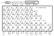
  Parallel pipeline structure of CMAC neural network. This learning algorithm can converge in one step.

See also[]

This "see also" section may contain an excessive number of suggestions. Please ensure that only the most relevant links are given, that they are not red links, and that any links are not already in this article. (March 2018) (Learn how and when to remove this template message)

References[]

Bibliography[]

External links[]

• The Neural Network Zoo – a compilation of neural network types
• The Stilwell Brain – a Mind Field episode featuring an experiment in which humans act as individual neurons in a neural network that classifies handwritten digits