Centripetal Catmull–Rom spline

In computer graphics, the centripetal Catmull–Rom spline is a variant form of the Catmull-Rom spline, originally formulated by Edwin Catmull and Raphael Rom,^[1] which can be evaluated using a recursive algorithm proposed by Barry and Goldman.^[2] It is a type of interpolating spline (a curve that goes through its control points) defined by four control points ${\displaystyle \mathbf {P} _{0},\mathbf {P} _{1},\mathbf {P} _{2},\mathbf {P} _{3}}$, with the curve drawn only from ${\displaystyle \mathbf {P} _{1}}$ to ${\displaystyle \mathbf {P} _{2}}$.

Catmull–Rom spline interpolation with four points

Definition[]

Barry and Goldman's pyramidal formulation

Knot parameterization for the Catmull–Rom algorithm

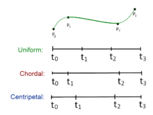
Let ${\displaystyle \mathbf {P} _{i}=[x_{i}\quad y_{i}]^{T}}$ denote a point. For a curve segment ${\displaystyle \mathbf {C} }$ defined by points ${\displaystyle \mathbf {P} _{0},\mathbf {P} _{1},\mathbf {P} _{2},\mathbf {P} _{3}}$ and knot sequence ${\displaystyle t_{0},t_{1},t_{2},t_{3}}$, the centripetal Catmull–Rom spline can be produced by:

${\displaystyle \mathbf {C} ={\frac {t_{2}-t}{t_{2}-t_{1}}}\mathbf {B} _{1}+{\frac {t-t_{1}}{t_{2}-t_{1}}}\mathbf {B} _{2}}$

where

${\displaystyle \mathbf {B} _{1}={\frac {t_{2}-t}{t_{2}-t_{0}}}\mathbf {A} _{1}+{\frac {t-t_{0}}{t_{2}-t_{0}}}\mathbf {A} _{2}}$

${\displaystyle \mathbf {B} _{2}={\frac {t_{3}-t}{t_{3}-t_{1}}}\mathbf {A} _{2}+{\frac {t-t_{1}}{t_{3}-t_{1}}}\mathbf {A} _{3}}$

${\displaystyle \mathbf {A} _{1}={\frac {t_{1}-t}{t_{1}-t_{0}}}\mathbf {P} _{0}+{\frac {t-t_{0}}{t_{1}-t_{0}}}\mathbf {P} _{1}}$

${\displaystyle \mathbf {A} _{2}={\frac {t_{2}-t}{t_{2}-t_{1}}}\mathbf {P} _{1}+{\frac {t-t_{1}}{t_{2}-t_{1}}}\mathbf {P} _{2}}$

${\displaystyle \mathbf {A} _{3}={\frac {t_{3}-t}{t_{3}-t_{2}}}\mathbf {P} _{2}+{\frac {t-t_{2}}{t_{3}-t_{2}}}\mathbf {P} _{3}}$

and

${\displaystyle t_{i+1}=\left[{\sqrt {(x_{i+1}-x_{i})^{2}+(y_{i+1}-y_{i})^{2}}}\right]^{\alpha }+t_{i}}$

in which ${\displaystyle \alpha }$ ranges from 0 to 1 for knot parameterization, and ${\displaystyle i=0,1,2,3}$ with ${\displaystyle t_{0}=0}$. For centripetal Catmull–Rom spline, the value of ${\displaystyle \alpha }$ is ${\displaystyle 0.5}$. When ${\displaystyle \alpha =0}$, the resulting curve is the standard ; when ${\displaystyle \alpha =1}$, the product is a .

Gif animation for uniform, centripetal and chordal parameterization of Catmull–Rom spline depending on the α value

Plugging ${\displaystyle t=t_{1}}$ into the spline equations ${\displaystyle \mathbf {A} _{1},\mathbf {A} _{2},\mathbf {A} _{3},\mathbf {B} _{1},\mathbf {B} _{2},}$ and ${\displaystyle \mathbf {C} }$ shows that the value of the spline curve at ${\displaystyle t_{1}}$ is ${\displaystyle \mathbf {C} =\mathbf {P} _{1}}$. Similarly, substituting ${\displaystyle t=t_{2}}$ into the spline equations shows that ${\displaystyle \mathbf {C} =\mathbf {P} _{2}}$ at ${\displaystyle t_{2}}$. This is true independent of the value of ${\displaystyle \alpha }$ since the equation for ${\displaystyle t_{i+1}}$ is not needed to calculate the value of ${\displaystyle \mathbf {C} }$ at points ${\displaystyle t_{1}}$ and ${\displaystyle t_{2}}$.

3D centripetal Catmull-Rom spline segment.

The extension to 3D points is simply achieved by considering ${\displaystyle \mathbf {P} _{i}=[x_{i}\quad y_{i}\quad z_{i}]^{T}}$a generic 3D point ${\displaystyle \mathbf {P} _{i}}$ and

${\displaystyle t_{i+1}=\left[{\sqrt {(x_{i+1}-x_{i})^{2}+(y_{i+1}-y_{i})^{2}+(z_{i+1}-z_{i})^{2}}}\right]^{\alpha }+t_{i}}$

Advantages[]

Centripetal Catmull–Rom spline has several desirable mathematical properties compared to the original and the other types of Catmull-Rom formulation.^[3] First, it will not form loop or self-intersection within a curve segment. Second, cusp will never occur within a curve segment. Third, it follows the control points more tightly.^[4][vague]

In this figure, there is a self-intersection/loop on the uniform Catmull-Rom spline (green), whereas for chordal Catmull-Rom spline (red), the curve does not follow tightly through the control points.

Other uses[]

In computer vision, centripetal Catmull-Rom spline has been used to formulate an active model for segmentation. The method is termed active spline model.^[5] The model is devised on the basis of active shape model, but uses centripetal Catmull-Rom spline to join two successive points (active shape model uses simple straight line), so that the total number of points necessary to depict a shape is less. The use of centripetal Catmull-Rom spline makes the training of a shape model much simpler, and it enables a better way to edit a contour after segmentation.

Code example in Python[]

The following is an implementation of the Catmull–Rom spline in Python that produces the plot shown beneath.

import numpy
import matplotlib.pyplot as plt

def CatmullRomSpline(P0, P1, P2, P3, nPoints=100):
    """
    P0, P1, P2, and P3 should be (x,y) point pairs that define the Catmull-Rom spline.
    nPoints is the number of points to include in this curve segment.
    """
    # Convert the points to numpy so that we can do array multiplication
    P0, P1, P2, P3 = map(numpy.array, [P0, P1, P2, P3])

    # Parametric constant: 0.5 for the centripetal spline, 0.0 for the uniform spline, 1.0 for the chordal spline.
    alpha = 0.5
    # Premultiplied power constant for the following tj() function.
    alpha = alpha/2
    def tj(ti, Pi, Pj):
        xi, yi = Pi
        xj, yj = Pj
        return ((xj-xi)**2 + (yj-yi)**2)**alpha + ti

    # Calculate t0 to t4
    t0 = 0
    t1 = tj(t0, P0, P1)
    t2 = tj(t1, P1, P2)
    t3 = tj(t2, P2, P3)

    # Only calculate points between P1 and P2
    t = numpy.linspace(t1, t2, nPoints)

    # Reshape so that we can multiply by the points P0 to P3
    # and get a point for each value of t.
    t = t.reshape(len(t), 1)
    print(t)
    A1 = (t1-t)/(t1-t0)*P0 + (t-t0)/(t1-t0)*P1
    A2 = (t2-t)/(t2-t1)*P1 + (t-t1)/(t2-t1)*P2
    A3 = (t3-t)/(t3-t2)*P2 + (t-t2)/(t3-t2)*P3
    print(A1)
    print(A2)
    print(A3)
    B1 = (t2-t)/(t2-t0)*A1 + (t-t0)/(t2-t0)*A2
    B2 = (t3-t)/(t3-t1)*A2 + (t-t1)/(t3-t1)*A3

    C = (t2-t)/(t2-t1)*B1 + (t-t1)/(t2-t1)*B2
    return C

def CatmullRomChain(P):
    """
    Calculate Catmull-Rom for a chain of points and return the combined curve.
    """
    sz = len(P)

    # The curve C will contain an array of (x, y) points.
    C = []
    for i in range(sz-3):
        c = CatmullRomSpline(P[i], P[i+1], P[i+2], P[i+3])
        C.extend(c)

    return C

# Define a set of points for curve to go through
Points = [[0, 1.5], [2, 2], [3, 1], [4, 0.5], [5, 1], [6, 2], [7, 3]]

# Calculate the Catmull-Rom splines through the points
c = CatmullRomChain(Points)

# Convert the Catmull-Rom curve points into x and y arrays and plot
x, y = zip(*c)
plt.plot(x, y)

# Plot the control points
px, py = zip(*Points)
plt.plot(px, py, 'or')

plt.show()

Plot obtained by the Python example code given above

Code example in Unity C#[]

using UnityEngine;

// a single catmull-rom curve
public struct CatmullRomCurve {

	public Vector2 p0, p1, p2, p3;
	public float alpha;

	public CatmullRomCurve( Vector2 p0, Vector2 p1, Vector2 p2, Vector2 p3, float alpha ) {
		( this.p0, this.p1, this.p2, this.p3 ) = ( p0, p1, p2, p3 );
		this.alpha = alpha;
	}

	// Evaluates a point at the given t-value from 0 to 1
	public Vector2 GetPoint( float t ) {
		// calculate knots
		const float k0 = 0;
		float k1 = GetKnotInterval( p0, p1 );
		float k2 = GetKnotInterval( p1, p2 ) + k1;
		float k3 = GetKnotInterval( p2, p3 ) + k2;

		// evaluate the point
		float u = Mathf.LerpUnclamped( k1, k2, t );
		Vector2 A1 = Remap( k0, k1, p0, p1, u );
		Vector2 A2 = Remap( k1, k2, p1, p2, u );
		Vector2 A3 = Remap( k2, k3, p2, p3, u );
		Vector2 B1 = Remap( k0, k2, A1, A2, u );
		Vector2 B2 = Remap( k1, k3, A2, A3, u );
		return Remap( k1, k2, B1, B2, u );
	}

	static Vector2 Remap( float a, float b, Vector2 c, Vector2 d, float u ) {
		return Vector2.LerpUnclamped( c, d, ( u - a ) / ( b - a ) );
	}

	float GetKnotInterval( Vector2 a, Vector2 b ) {
		return Mathf.Pow( Vector2.SqrMagnitude( a - b ), 0.5f * alpha );
	}

}

using UnityEngine;

// Draws a catmull-rom spline in the scene view,
// along the child objects of the transform of this component
public class CatmullRomSpline : MonoBehaviour {

	[Range( 0, 1 )] public float alpha = 0.5f;
	int PointCount => transform.childCount;
	int SegmentCount => PointCount - 3;
	Vector2 GetPoint( int i ) => transform.GetChild( i ).position;

	CatmullRomCurve GetCurve( int i ) {
		return new CatmullRomCurve( GetPoint(i), GetPoint(i+1), GetPoint(i+2), GetPoint(i+3), alpha );
	}

	void OnDrawGizmos() {
		for( int i = 0; i < SegmentCount; i++ )
			DrawCurveSegment( GetCurve( i ) );
	}

	void DrawCurveSegment( CatmullRomCurve curve ) {
		const int detail = 32;
		Vector2 prev = curve.p1;
		for( int i = 1; i < detail; i++ ) {
			float t = i / ( detail - 1f );
			Vector2 pt = curve.GetPoint( t );
			Gizmos.DrawLine( prev, pt );
			prev = pt;
		}
	}
}

Code example in Unreal C++[]

float GetT( float t, float alpha, const FVector& p0, const FVector& p1 )
{
    auto d  = p1 - p0;
    float a = d | d; // Dot product
    float b = FMath::Pow( a, alpha*.5f );
    return (b + t);
}

FVector CatmullRom( const FVector& p0, const FVector& p1, const FVector& p2, const FVector& p3, float t /* between 0 and 1 */, float alpha=.5f /* between 0 and 1 */ )
{
    float t0 = 0.0f;
    float t1 = GetT( t0, alpha, p0, p1 );
    float t2 = GetT( t1, alpha, p1, p2 );
    float t3 = GetT( t2, alpha, p2, p3 );
    t = FMath::Lerp( t1, t2, t );
    FVector A1 = ( t1-t )/( t1-t0 )*p0 + ( t-t0 )/( t1-t0 )*p1;
    FVector A2 = ( t2-t )/( t2-t1 )*p1 + ( t-t1 )/( t2-t1 )*p2;
    FVector A3 = ( t3-t )/( t3-t2 )*p2 + ( t-t2 )/( t3-t2 )*p3;
    FVector B1 = ( t2-t )/( t2-t0 )*A1 + ( t-t0 )/( t2-t0 )*A2;
    FVector B2 = ( t3-t )/( t3-t1 )*A2 + ( t-t1 )/( t3-t1 )*A3;
    FVector C  = ( t2-t )/( t2-t1 )*B1 + ( t-t1 )/( t2-t1 )*B2;
    return C;
}

See also[]

• Cubic Hermite splines

References[]

External links[]

• Catmull-Rom curve with no cusps and no self-intersections – implementation in Java
• Catmull-Rom curve with no cusps and no self-intersections – simplified implementation in C++
• Catmull-Rom splines – interactive generation via Python, in a Jupyter notebook