Hill equation (biochemistry)

Binding curves showing the characteristically sigmoidal curves generated by using the Hill–Langmuir equation to model cooperative binding. Each curve corresponds to a different Hill coefficient, labeled to the curve's right. The vertical axis displays the proportion of the total number of receptors that have been bound by a ligand. The horizontal axis is the concentration of the ligand. As the Hill coefficient is increased, the saturation curve becomes steeper.

In biochemistry and pharmacology, the Hill equation refers to two closely related equations that reflect the binding of ligands to macromolecules, as a function of the ligand concentration. A ligand is "a substance that forms a complex with a biomolecule to serve a biological purpose" (ligand definition), and a macromolecule is a very large molecule, such as a protein, with a complex structure of components (macromolecule definition). Protein-ligand binding typically changes the structure of the target protein, thereby changing its function in a cell.

The distinction between the two Hill equations is whether they measure occupancy or response. The Hill–Langmuir equation reflects the occupancy of macromolecules: the fraction that is saturated or bound by the ligand.^{[1][2][nb 1]} This equation is formally equivalent to the Langmuir isotherm.^[3] Conversely, the Hill equation proper reflects the cellular or tissue response to the ligand: the physiological output of the system, such as muscle contraction.

The Hill–Langmuir equation was originally formulated by Archibald Hill in 1910 to describe the sigmoidal O₂ binding curve of haemoglobin.^[4]

The binding of a ligand to a macromolecule is often enhanced if there are already other ligands present on the same macromolecule (this is known as cooperative binding). The Hill–Langmuir equation is useful for determining the degree of cooperativity of the ligand(s) binding to the enzyme or receptor. The Hill coefficient provides a way to quantify the degree of interaction between ligand binding sites.^[5]

The Hill equation (for response) is important in the construction of dose-response curves.

Proportion of ligand-bound receptors[]

Plot of the % saturation of oxygen binding to haemoglobin, as a function of the amount of oxygen present (expressed as an oxygen pressure). Data (red circles) and Hill equation fit (black curve) from original 1910 paper of Hill.^[6]

The Hill–Langmuir equation is a special case of a rectangular hyperbola and is commonly expressed in the following ways.^[2][7][8]

${\displaystyle {\begin{aligned}\theta &={[{\ce {L}}]^{n} \over K_{d}+[{\ce {L}}]^{n}}\\&={[{\ce {L}}]^{n} \over (K_{A})^{n}+[{\ce {L}}]^{n}}\\&={1 \over 1+\left({K_{A} \over [{\ce {L}}]}\right)^{n}}\end{aligned}}}$,

where:

• ${\displaystyle \theta }$ is the fraction of the receptor protein concentration that is bound by the ligand,
• ${\displaystyle {\ce {[L]}}}$is the total ligand concentration,
• ${\displaystyle K_{d}}$ is the apparent dissociation constant derived from the law of mass action,
• ${\displaystyle K_{A}}$is the ligand concentration producing half occupation,
• ${\displaystyle n}$ is the Hill coefficient.

Constants[]

In pharmacology, ${\displaystyle \theta }$ is often written as ${\displaystyle p_{AR}}$, where ${\displaystyle A}$ is the ligand, equivalent to L, and ${\displaystyle R}$ is the receptor. ${\displaystyle \theta }$ can be expressed in terms of the total amount of receptor and ligand-bound receptor concentrations: ${\displaystyle \theta ={\frac {[LR]}{[R_{\rm {total}}]}}}$. ${\displaystyle K_{d}}$ is equal to the ratio of the dissociation rate of the ligand-receptor complex to its association rate (${\textstyle K_{\rm {d}}={k_{\rm {d}} \over k_{\rm {a}}}}$).^[8] Kd is the equilibrium constant for dissociation. ${\textstyle K_{A}}$ is defined so that ${\textstyle (K_{A})^{n}=K_{\rm {d}}={k_{\rm {d}} \over k_{\rm {a}}}}$, this is also known as the microscopic dissociation constant and is the ligand concentration occupying half of the binding sites. In recent literature, this constant is sometimes referred to as ${\textstyle K_{D}}$.^[8]

Gaddum equation[]

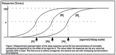
The Gaddum equation is a further generalisation of the Hill-equation, incorporating the presence of a reversible competitive antagonist.^[1] The Gaddum equation is derived similarly to the Hill-equation but with 2 equilibria: both the ligand with the receptor and the antagonist with the receptor. Hence, the Gaddum equation has 2 constants: the equilibrium constants of the ligand and that of the antagonist

Hill plot[]

A Hill plot, where the x-axis is the logarithm of the ligand concentration and the y-axis is the transformed receptor occupancy. X represents L and Y represents theta.

The Hill plot is the rearrangement of the Hill–Langmuir Equation into a straight line.

Taking the reciprocal of both sides of the Hill–Langmuir equation, rearranging, and inverting again yields: ${\displaystyle {\theta \over 1-\theta }={[{\ce {L}}]^{n} \over K_{d}}={[{\ce {L}}]^{n} \over (K_{A})^{n}}}$. Taking the logarithm of both sides of the equation leads to an alternative formulation of the Hill-Langmuir equation:

${\displaystyle {\begin{aligned}\log \left({\theta \over 1-\theta }\right)&=n\log {[{\ce {L}}]}-\log {K_{d}}\\&=n\log {[{\ce {L}}]}-n\log {K_{A}}\end{aligned}}}$.

This last form of the Hill–Langmuir equation is advantageous because a plot of ${\textstyle \log \left({\theta \over 1-\theta }\right)}$ versus ${\displaystyle \log {[{\ce {L}}]}}$ yields a linear plot, which is called a Hill plot.^[7][8] Because the slope of a Hill plot is equal to the Hill coefficient for the biochemical interaction, the slope is denoted by ${\displaystyle n_{H}}$. A slope greater than one thus indicates positively cooperative binding between the receptor and the ligand, while a slope less than one indicates negatively cooperative binding.

Transformations of equations into linear forms such as this were very useful before the widespread use of computers, as they allowed researchers to determine parameters by fitting lines to data. However, these transformations affect error propagation, and this may result in undue weight to error in data points near 0 or 1.^{[nb 2]} This impacts the parameters of linear regression lines fitted to the data. Furthermore, the use of computers enables more robust analysis involving nonlinear regression.

Tissue response[]

A trio of dose response curves

A distinction should be made between quantification of drugs binding to receptors and drugs producing responses. There may not necessarily be a linear relationship between the two values. In contrast to this article's previous definition of the Hill-Langmuir equation, the IUPHAR defines the Hill equation in terms of the tissue response ${\displaystyle (E)}$, as

${\displaystyle {\begin{aligned}{\frac {E}{E_{\mathrm {max} }}}&={\frac {[A]^{n}}{{\text{EC}}_{50}^{n}+[A]^{n}}}\\&={\frac {1}{1+\left({\frac {{\text{EC}}_{50}}{[A]}}\right)^{n}}}\end{aligned}}}$^[1]

where ${\displaystyle {\ce {[A]}}}$ is the drug concentration and ${\displaystyle {\text{EC}}_{50}}$ is the drug concentration that produces a 50% maximal response. Dissociation constants (in the previous section) relate to ligand binding, while ${\displaystyle {\text{EC}}_{50}}$ reflects tissue response.

This form of the equation can reflect tissue/cell/population responses to drugs and can be used to generate dose response curves. The relationship between ${\displaystyle K_{d}}$ and EC50 may be quite complex as a biological response will be the sum of myriad factors; a drug will have a different biological effect if more receptors are present, regardless of its affinity.

The Del-Castillo Katz model is used to relate the Hill–Langmuir equation to receptor activation by including a second equilibrium of the ligand-bound receptor to an activated form of the ligand-bound receptor.

Statistical analysis of response as a function of stimulus may be performed by regression methods such as the probit model or logit model, or other methods such as the .^[9] Empirical models based on nonlinear regression are usually preferred over the use of some transformation of the data that linearizes the dose-response relationship.^[10]

Hill coefficient[]

The Hill coefficient is a measure of ultrasensitivity (i.e. how steep is the response curve).

The Hill coefficient, ${\displaystyle n}$ or ${\displaystyle n_{H}}$, may describe cooperativity (or possibly other biochemical properties, depending on the context in which the Hill–Langmuir equation is being used). When appropriate,^{[clarification needed]} the value of the Hill coefficient describes the cooperativity of ligand binding in the following way:

• ${\displaystyle n>1}$. Positively cooperative binding: Once one ligand molecule is bound to the enzyme, its affinity for other ligand molecules increases. For example, the Hill coefficient of oxygen binding to haemoglobin (an example of positive cooperativity) falls within the range of 1.7–3.2.^[5]
• ${\displaystyle n<1}$. Negatively cooperative binding: Once one ligand molecule is bound to the enzyme, its affinity for other ligand molecules decreases.
• ${\displaystyle n=1}$. Noncooperative (completely independent) binding: The affinity of the enzyme for a ligand molecule is not dependent on whether or not other ligand molecules are already bound. When n=1, we obtain a model that can be modeled by Michaelis–Menten kinetics,^[11] in which ${\textstyle K_{D}=K_{A}=K_{M}}$, the Michaelis–Menten constant.

The Hill coefficient can be calculated in terms of potency as:

${\displaystyle n_{H}={\frac {\log _{10}(81)}{\log _{10}({\ce {EC90}}/{\ce {EC10}})}}}$.^[12]

where ${\displaystyle {\ce {EC90}}}$ and ${\displaystyle {\ce {EC10}}}$ are the input values needed to produce the 10% and 90% of the maximal response, respectively.^[13]

Derivation from mass action kinetics[]

The Hill-Langmuir equation is derived similarly to the Michaelis Menten equation^[14][15] but incorporates the Hill coefficient. Consider a protein (${\displaystyle P}$), such as haemoglobin or a protein receptor, with ${\displaystyle {\mathit {n}}}$ binding sites for ligands (${\displaystyle L}$). The binding of the ligands to the protein can be represented by the chemical equilibrium expression:

${\displaystyle {\ce {{P}+{\mathit {n}}{L}<=>[k_{a}][k_{d}]{P}{L}_{\mathit {n}}}}}$,

where ${\displaystyle k_{a}}$ (forward rate, or the rate of association of the protein-ligand complex) and ${\displaystyle k_{d}}$ (reverse rate, or the complex's rate of dissociation) are the reaction rate constants for the association of the ligands to the protein and their dissociation from the protein, respectively.^[8] From the law of mass action, which in turn may be derived from the principles of collision theory, the apparent dissociation constant ${\displaystyle K_{d}}$, an equilibrium constant, is given by:

${\displaystyle K_{\rm {d}}={k_{\rm {d}} \over k_{\rm {a}}}={{[{\rm {P}}][{\rm {L}}]^{\mathit {n}}} \over [{\rm {PL_{\mathit {n}}}}]}}$.

At the same time, ${\displaystyle \theta }$, the ratio of the concentration of occupied receptor to total receptor concentration, is given by:

${\displaystyle \theta ={\mathrm {Occupied\ Receptor} \over \mathrm {Total\ Receptor} }={[{\rm {PL_{\mathit {n}}}}] \over {[{\rm {P}}]\ +\ [{\rm {PL_{\mathit {n}}}}]}}}$.

By using the expression obtained earlier for the dissociation constant, we can replace ${\textstyle [{\rm {PL_{\mathit {n}}}}]}$ with ${\textstyle {[{\rm {P}}][{\rm {L}}]^{\mathit {n}} \over K_{\rm {d}}}}$ to yield a simplified expression for ${\textstyle \theta }$:

${\displaystyle \theta ={({[{\rm {P}}][{\rm {L}}]^{\mathit {n}} \over K_{\rm {d}}}) \over {[{\rm {P}}]\ +\ ({[{\rm {P}}][{\rm {L}}]^{\mathit {n}} \over K_{\rm {d}}})}}={{[{\rm {P}}][{\rm {L}}]^{\mathit {n}}} \over {K_{\rm {d}}[{\rm {P}}]\ +\ {[{\rm {P}}][{\rm {L}}]^{\mathit {n}}}}}={{[{\rm {L}}]^{\mathit {n}}} \over {K_{\rm {d}}\ +\ {[{\rm {L}}]^{\mathit {n}}}}}}$,

which is a common formulation of the Hill equation.^[7][16][8]

Assuming that the protein receptor was initially completely free (unbound) at a concentration ${\textstyle [{\rm {P_{0}}}]}$, then at any time, ${\textstyle {[{\rm {P}}]+[{\rm {PL_{\mathit {n}}}}]}=[{\rm {P_{0}}}]}$ and ${\textstyle \theta ={[{\rm {PL_{\mathit {n}}}}] \over {[{\rm {P_{0}}}]\ }}}$. Consequently, the Hill–Langmuir Equation is also commonly written as an expression for the concentration ${\textstyle [{\rm {PL_{\mathit {n}}}}]}$of bound protein:

${\displaystyle [{\rm {PL_{\mathit {n}}}}]=[{\rm {P_{0}}}]\cdot {{[{\rm {L}}]^{\mathit {n}}} \over {K_{\rm {d}}\ +\ {[{\rm {L}}]^{\mathit {n}}}}}}$ .^[2]

All of these formulations assume that the protein has ${\displaystyle {\mathit {n}}}$ sites to which ligands can bind. In practice, however, the Hill Coefficient ${\displaystyle {\mathit {n}}}$ rarely provides an accurate approximation of the number of ligand binding sites on a protein.^[5][7] Consequently, it has been observed that the Hill coefficient should instead be interpreted as an "interaction coefficient" describing the cooperativity among ligand binding sites.^[5]

Applications[]

The Hill and Hill–Langmuir equations are used extensively in pharmacology to quantify the functional parameters of a drug^{[citation needed]} and are also used in other areas of biochemistry.

The Hill equation can be used to describe dose-response relationships, for example ion channel open-probability (P-open) vs. ligand concentration.^[17]

Regulation of gene transcription[]

The Hill–Langmuir equation can be applied in modelling the rate at which a gene product is produced when its parent gene is being regulated by transcription factors (e.g., activators and/or repressors).^[11] Doing so is appropriate when a gene is regulated by multiple binding sites for transcription factors, in which case the transcription factors may bind the DNA in a cooperative fashion.^[18]

If the production of protein from gene X is up-regulated (activated) by a transcription factor Y, then the rate of production of protein X can be modeled as a differential equation in terms of the concentration of activated Y protein:

${\displaystyle {\mathrm {d} \over \mathrm {d} t}[{\rm {X_{produced}}}]=k\ \cdot {{[{\rm {Y_{active}}}]^{\mathit {n}}} \over {(K_{A})^{n}\ +\ {[{\rm {Y_{active}}}]^{\mathit {n}}}}}}$,

where k is the maximal transcription rate of gene X.

Likewise, if the production of protein from gene Y is down-regulated (repressed) by a transcription factor Z, then the rate of production of protein Y can be modeled as a differential equation in terms of the concentration of activated Z protein:

${\displaystyle {\mathrm {d} \over \mathrm {d} t}[{\rm {Y_{produced}}}]=k\ \cdot {{(K_{A})^{\mathit {n}}} \over {(K_{A})^{n}\ +\ {[{\rm {Z_{active}}}]^{\mathit {n}}}}}}$,

where k is the maximal transcription rate of gene Y.

Limitations[]

Because of its assumption that ligand molecules bind to a receptor simultaneously, the Hill–Langmuir equation has been criticized as a physically unrealistic model.^[5] Moreover, the Hill coefficient should not be considered a reliable approximation of the number of cooperative ligand binding sites on a receptor^[5][19] except when the binding of the first and subsequent ligands results in extreme positive cooperativity.^[5]

Unlike more complex models, the relatively simple Hill–Langmuir equation provides little insight into underlying physiological mechanisms of protein-ligand interactions. This simplicity, however, is what makes the Hill–Langmuir equation a useful empirical model, since its use requires little a priori knowledge about the properties of either the protein or ligand being studied.^[2] Nevertheless, other, more complex models of cooperative binding have been proposed.^[7] For more information and examples of such models, see Cooperative binding.

Global sensitivity measure such as Hill coefficient do not characterise the local behaviours of the s-shaped curves. Instead, these features are well captured by the response coefficient measure.^[20]

There is a link between Hill Coefficient and Response coefficient, as follows. Altszyler et al. (2017) have shown that these ultrasensitivity measures can be linked.^[12]

See also[]

• Bjerrum plot
• Cooperative binding
• Gompertz curve
• Langmuir adsorption model
• Logistic function
• Michaelis–Menten kinetics
• Monod equation

Notes[]

References[]

Further reading[]

• Dorland's Illustrated Medical Dictionary
• Coval, ML (December 1970). "Analysis of Hill interaction coefficients and the invalidity of the Kwon and Brown equation". J. Biol. Chem. 245 (23): 6335–6. doi:10.1016/S0021-9258(18)62614-6. PMID 5484812.
• d'A Heck, Henry (1971). "Statistical theory of cooperative binding to proteins. Hill equation and the binding potential". J. Am. Chem. Soc. 93 (1): 23–29. doi:10.1021/ja00730a004. PMID 5538860.
• Atkins, Gordon L. (1973). "A simple digital-computer program for estimating the parameter of the Hill Equation". Eur. J. Biochem. 33 (1): 175–180. doi:10.1111/j.1432-1033.1973.tb02667.x. PMID 4691349.
• Endrenyi, Laszlo; Kwong, F. H. F.; Fajszi, Csaba (1975). "Evaluation of Hill slopes and Hill coefficients when the saturation binding or velocity is not known". Eur. J. Biochem. 51 (2): 317–328. doi:10.1111/j.1432-1033.1975.tb03931.x. PMID 1149734.
• Voet, Donald; Voet, Judith G. Biochemistry.
• Weiss, J. N. (1997). "The Hill equation revisited: uses and misuses". FASEB Journal. 11 (11): 835–841. doi:10.1096/fasebj.11.11.9285481. PMID 9285481. S2CID 827335.
• Kurganov, B. I.; Lobanov, A. V. (2001). "Criterion for Hill equation validity for description of biosensor calibration curves". Anal. Chim. Acta. 427 (1): 11–19. doi:10.1016/S0003-2670(00)01167-3.
• Goutelle, Sylvain; Maurin, Michel; Rougier, Florent; Barbaut, Xavier; Bourguignon, Laurent; Ducher, Michel; Maire, Pascal (2008). "The Hill equation: a review of its capabilities in pharmacological modelling". Fundamental & Clinical Pharmacology. 22 (6): 633–648. doi:10.1111/j.1472-8206.2008.00633.x. PMID 19049668. S2CID 4979109.
• Gesztelyi R; Zsuga J; Kemeny-Beke A; Varga B; Juhasz B; Tosaki A (2012). "The Hill equation and the origin of quantitative pharmacology". Archive for History of Exact Sciences. 66 (4): 427–38. doi:10.1007/s00407-012-0098-5. S2CID 122929930.
• Colquhoun D (2006). "The quantitative analysis of drug-receptor interactions: a short history". Trends Pharmacol Sci. 27 (3): 149–57. doi:10.1016/j.tips.2006.01.008. PMID 16483674.
• Rang HP (2006). "The receptor concept: pharmacology's big idea". Br J Pharmacol. 147: S9–16. doi:10.1038/sj.bjp.0706457. PMC 1760743. PMID 16402126.

External links[]

• Hill equation calculator