Interquartile range
This article needs additional citations for verification. (May 2012) |

In descriptive statistics, the interquartile range (IQR) is a measure of statistical dispersion. It is the spread of the data or observations.[1] The IQR may also be called the midspread, middle 50%, or H‑spread. It is defined as the spread difference between the 75th and 25th percentiles of the data.[2][3][4] To calculate the IQR, the data set is divided into quartiles, or four rank-ordered even parts via linear interpolation.[1] These quartiles are denoted by Q1 (also called the lower quartile), Q2 (the median), and Q3 (also called the upper quartile). The lower quartile corresponds with the 25th percentile and the upper quartile corresponds with the 75th percentile, so IQR = Q3 − Q1.[1]
The IQR is an example of a trimmed estimator, defined as the 25% trimmed range, which enhances the accuracy of dataset statistics by dropping lower contribution, outlying points.[5] It is also used as a robust measure of scale[5] IQR spread can be clearly visualized by the box on a Box plot.[1]
Use[]
The primary use of the IQR is to represent the spread difference between the upper and lower quartiles of a data set. This can be used as an indicator for variability of the dataset.[1]
It is also used to build box plots, which are a graphical representation of probability distribution. In the box plot, the IQR is the height of the box itself, and the whiskers have a length of 1.5*IQR.[1] Any data point located outside of the whiskers is referred to as an outlier (see below).[1]
MAD or total range or median absolute deviation is often used as a preferred measurement or variability to IQR because IQR has a lower breakdown point: 25%, compared to MAD's 50%, where 50% is the optimum. [6]
The IQR has been practically used in a number of recent studies. Some of these uses include:
Algorithm[]
Discrete Variables[]
The IQR of a set of values is calculated as the difference between the upper and lower quartiles, Q3 and Q1. Each quartile is a median calculated as follows.
Given an even 2n or odd 2n+1 number of values:
- first quartile Q1 = median of the n smallest values;
- third quartile Q3 = median of the n largest values.[10]
The second quartile Q2 is the same as the ordinary median.[10]
Continuous Variables[]
The interquartile range of a continuous distribution can be calculated by integrating the probability density function (PDF) over specific intervals. The lower quartile, Q1, is a number such that integral of the PDF from -∞ to Q1 equals 0.25, while the upper quartile, Q3, is such a number that the integral from -∞ to Q3 equals 0.75.[1]
In terms of the CDF, the quartiles can be defined as follows: where CDF−1 is the quantile function.[1]
This article is missing information about CDF. (February 2022) |
Examples[]
Data set in a table[]
The following table has 13 rows, and follows the rules for the odd number of entries.
| i | x[i] | Median | Quartile |
|---|---|---|---|
| 1 | 7 | Q2 = 87 (median of whole table) |
Q1 = 31 (median of upper half, from row 1 to 6) |
| 2 | 7 | ||
| 3 | 31 | ||
| 4 | 31 | ||
| 5 | 47 | ||
| 6 | 75 | ||
| 7 | 87 | ||
| 8 | 115 | ||
| Q3 = 119 (median of lower half, from row 8 to 13) | |||
| 9 | 116 | ||
| 10 | 119 | ||
| 11 | 119 | ||
| 12 | 155 | ||
| 13 | 177 |
For the data in this table the interquartile range is IQR = Q3 − Q1 = 119 - 31 = 88.
Data set in a plain-text box plot[]
                             +−−−−−+−+
               * |−−−−−−−−−−−|     | |−−−−−−−−−−−|
                             +−−−−−+−+

 +−−−+−−−+−−−+−−−+−−−+−−−+−−−+−−−+−−−+−−−+−−−+−−−+   number line
 0   1   2   3   4   5   6   7   8   9   10  11  12
For the data set in this box plot:
- lower (first) quartile Q1 = 7
- median (second quartile) Q2 = 8.5
- upper (third) quartile Q3 = 9
- interquartile range, IQR = Q3 - Q1 = 2
- lower 1.5*IQR whisker = Q1 - 1.5 * IQR = 7 - 3 = 4. (If there is no data point at 4, then the lowest point greater than 4.)
- upper 1.5*IQR whisker = Q3 + 1.5 * IQR = 9 + 3 = 12. (If there is no data point at 12, then the highest point less than 12.)
This means the 1.5*IQR whiskers can be uneven in lengths. The median, minimum, maximum, and the first and third quartile constitute the Five-number summary.[1][11]
Distributions[]
The interquartile range and median of some common distributions are shown below:
| Distribution | Median | IQR |
|---|---|---|
| Normal | μ | 2 Φ−1(0.75)σ ≈ 1.349σ ≈ (27/20)σ |
| Laplace | μ | 2b ln(2) ≈ 1.386b |
| Cauchy | μ | 2γ |
If both the median and mean of a distribution fall inside the interquartile range, the distribution is considered to be reasonably symmetrical.[12]
Outliers[]
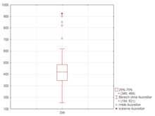
The interquartile range is often used to find outliers in data. A fence is used to identify and categorize types of outliers from the data, or on a box plot.[13] There are four relevant fences:
- Lower Inner Fence: Q1 - 1.5 * IQR
- Upper Inner Fence: Q3 + 1.5 * IQR
- Lower Outer Fence: Q1 - 3 * IQR
- Upper Outer Fence: Q3 + 3 * IQR
Any data points that fall between the inner and outer fences are called mild outliers. Points that fall beyond the outer fences are called extreme outliers.[13]
See also[]
- Interdecile range
- Midhinge
- Probable error
- Robust measures of scale
References[]
- ^ a b c d e f g h i j Dekking, Frederik Michel; Kraaikamp, Cornelis; Lopuhaä, Hendrik Paul; Meester, Ludolf Erwin (2005). A Modern Introduction to Probability and Statistics. Springer Texts in Statistics. London: Springer London. doi:10.1007/1-84628-168-7. ISBN 978-1-85233-896-1.
- ^ Upton, Graham; Cook, Ian (1996). Understanding Statistics. Oxford University Press. p. 55. ISBN 0-19-914391-9.
- ^ Zwillinger, D., Kokoska, S. (2000) CRC Standard Probability and Statistics Tables and Formulae, CRC Press. ISBN 1-58488-059-7 page 18.
- ^ Ross, Sheldon (2010). Introductory Statistics. Burlington, MA: Elsevier. pp. 103–104. ISBN 978-0-12-374388-6.
- ^ a b Kaltenbach, Hans-Michael (2012). A concise guide to statistics. Heidelberg: Springer. ISBN 978-3-642-23502-3. OCLC 763157853.
- ^ Rousseeuw, Peter J.; Croux, Christophe (1992). Y. Dodge (ed.). "Explicit Scale Estimators with High Breakdown Point" (PDF). L1-Statistical Analysis and Related Methods. Amsterdam: North-Holland. pp. 77–92.
- ^ Zhang, Yiming; Kim, Nam H.; Haftka, Raphael T. (2019-11-20). "General-Surrogate Adaptive Sampling Using Interquartile Range for Design Space Exploration". Journal of Mechanical Design. 142 (5). doi:10.1115/1.4044432. ISSN 1050-0472. S2CID 201235547.
- ^ Dai, Zhifeng and Xiaomin Chang. “Predicting Stock Return with Economic Constraint: Can Interquartile Range Truncate the Outliers?” (2021).
- ^ Ajil, Jassim, Firas (2013-02-05). Image Denoising Using Interquartile Range Filter with Local Averaging. OCLC 1106182050.
- ^ a b Bertil., Westergren (1988). Beta [beta] mathematics handbook : concepts, theorems, methods, algorithms, formulas, graphs, tables. Studentlitteratur. p. 348. ISBN 9144250517. OCLC 18454776.
- ^ Tukey, J.W. "Exploratory data analysis". Addison-Wesley, Reading, 1977.
- ^ Whitley, Elise; Ball, Jonathan (2002). "Statistics review 1: Presenting and summarising data". Critical Care. 6 (1): 66–71. doi:10.1186/cc1455. ISSN 1364-8535. PMC 137399. PMID 11940268.
- ^ a b "NIST/SEMATECH e-Handbook of Statistical Methods". www.itl.nist.gov. doi:10.18434/m32189. Retrieved 2021-12-14.
External links[]
 Media related to Interquartile range at Wikimedia Commons
Statistics | |||||||||||||||||||||||||||
|---|---|---|---|---|---|---|---|---|---|---|---|---|---|---|---|---|---|---|---|---|---|---|---|---|---|---|---|
| |||||||||||||||||||||||||||
| |||||||||||||||||||||||||||
| |||||||||||||||||||||||||||
| |||||||||||||||||||||||||||
| |||||||||||||||||||||||||||
| |||||||||||||||||||||||||||
| |||||||||||||||||||||||||||
| |||||||||||||||||||||||||||
- Scale statistics