Kelvin–Helmholtz instability

This article includes a list of general references, but it remains largely unverified because it lacks sufficient corresponding inline citations. Please help to improve this article by introducing more precise citations. (March 2010) (Learn how and when to remove this template message)

Play media

Numerical simulation of a temporal Kelvin–Helmholtz instability

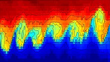
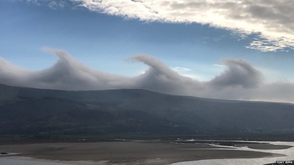
The Kelvin–Helmholtz instability (after Lord Kelvin and Hermann von Helmholtz) typically occurs when there is velocity shear in a single continuous fluid, or additionally where there is a velocity difference across the interface between two fluids. A common example is seen when wind blows across a water surface; the instability constant manifests as waves. Kelvin-Helmholtz instabilities are also visible in the atmospheres of planets and moons, such as in cloud formations on Earth or the Red Spot on Jupiter, and the atmospheres (coronas) of stars, including the sun's.^[1]

Spatially developing 2D Kelvin-Helmholtz instability at low Reynolds number. Small perturbations, imposed at the inlet on the tangential velocity, evolve in the computational box. High Reynolds number would be marked with an increase of small scale motions.

Theory overview and mathematical concepts[]

A KH instability rendered visible by clouds, known as fluctus,^[2] over Mount Duval in Australia

A KH instability on the planet Saturn, formed at the interaction of two bands of the planet's atmosphere

Kelvin-Helmholtz billows 500m deep in the Atlantic Ocean

Animation of the KH instability, using a second order 2D finite volume scheme

The theory predicts the onset of instability and transition to turbulent flow within fluids of different densities moving at various speeds.^[3] Helmholtz studied the dynamics of two fluids of different densities when a small disturbance, such as a wave, was introduced at the boundary connecting the fluids. Kelvin–Helmholtz instability can thus be characterized as unstable small scale motions occurring vertically and laterally. At times, the small scale instabilities can be limited through the presence of a boundary. The boundaries are evident in the vertical direction, through an upper and lower boundary. The upper boundary can be seen as through examples as the free surface of an ocean and lower boundary as a wave breaking on a coast.^[4] On a lateral scale, diffusion and viscosity are the main factors of considerations as both affect small-scale instabilities. Through the aforementioned definition of the Kelvin–Helmholtz instability, the distinction between Kelvin–Helmholtz instability and small scale turbulence can be difficult. Although the two are not inherently inseparable, Kelvin-Helmholtz is viewed as a two dimensional phenomenon compared to turbulence occurring in three dimensions.^[4]

In the case of a short wavelength, if surface tension is ignored, two fluids in parallel motion with different velocities and densities yield an interface that is unstable for all speeds. However, surface tension is able to stabilize the short wavelength instability and predict stability until a velocity threshold is reached. The linear stability theory, with surface tension included, broadly predicts the onset of wave formation as well as the transition to turbulence in the important case of wind over water.^[5]

It was recently discovered that the fluid equations governing the linear dynamics of the system admit a parity-time symmetry, and the Kelvin–Helmholtz instability occurs when and only when the parity-time symmetry breaks spontaneously.^[6]

For a continuously varying distribution of density and velocity (with the lighter layers uppermost, so that the fluid is RT-stable), the dynamics of the Kelvin-Helmholtz instability is described by the Taylor–Goldstein equation ${\displaystyle (U-c)[\psi -k^{2}\psi ]+\left[{\frac {N^{2}}{U-c}}-U\right]\psi =0}$ and its onset is given by the Richardson number ${\displaystyle \mathrm {Ri} }$.^[4] Typically the layer is unstable for ${\displaystyle \mathrm {Ri} <0.25}$. These effects are common in cloud layers. The study of this instability is applicable in plasma physics, for example in inertial confinement fusion and the plasma–beryllium interface. At times a situation in which there in a state of static stability, evident by heavier fluids found below than the lower fluid, the Rayleigh-Taylor instability can be ignored as the Kelvin–Helmholtz instability is sufficient given the conditions.

It is understood that in the case of small-scale turbulence, an increase of the Reynolds number, ${\displaystyle {\displaystyle \mathrm {Re} ={\frac {\rho uD}{\mu }}={\frac {uD}{\nu }}}}$, corresponds with an increase of small scale motions. Introducing the Reynolds number is comparable to introducing a measure of viscosity to a relationship that was previously defined as velocity shear and instability. In terms of viscosity, a high Reynolds number is denoted by low viscosity. Essentially, high Reynolds number results in the increase of small scale motion. This idea is considered to be in line with the nature of the Kelvin–Helmholtz instability.^[7] When increasing the Reynolds number within a case of the Kelvin–Helmholtz instability, the initial large-scale structures of the instability are shown to still persist in the form of supersonic forms.^[8]

Numerically, the Kelvin–Helmholtz instability is simulated in a temporal or a spatial approach. In the temporal approach, experimenters consider the flow in a periodic (cyclic) box "moving" at mean speed (absolute instability). In the spatial approach, experimenters simulate a lab experiment with natural inlet and outlet conditions (convective instability).

Importance and real-life applications[]

The Kelvin–Helmholtz instability phenomenon is an all encompassing occurrence of fluid flow seen time and time again in nature. From the waves of the ocean to the clouds above in the sky, the Kelvin–Helmholtz instability is responsible for some of nature's most basic structures. Further analysis and modeling of the Kelvin–Helmholtz instability can result in an understanding of the worlds natural phenomena and more.

See also[]

• Rayleigh–Taylor instability
• Richtmyer–Meshkov instability
• Mushroom cloud
• Plateau–Rayleigh instability
• Kármán vortex street
• Taylor–Couette flow
• Fluid mechanics
• Fluid dynamics
• Reynolds number
• Turbulence

Notes[]

References[]

• Lord Kelvin (William Thomson) (1871). "Hydrokinetic solutions and observations". Philosophical Magazine. 42: 362–377.
• Hermann von Helmholtz (1868). "Über discontinuierliche Flüssigkeits-Bewegungen [On the discontinuous movements of fluids]". Monatsberichte der Königlichen Preussische Akademie der Wissenschaften zu Berlin. 23: 215–228.
• Article describing discovery of K-H waves in deep ocean: Broad, William J. (April 19, 2010). "In Deep Sea, Waves With a Familiar Curl". New York Times. Retrieved April 23, 2010.

External links[]

Wikimedia Commons has media related to Kelvin-Helmholtz waves.

• Hwang, K.-J.; Goldstein; Kuznetsova; Wang; Viñas; Sibeck (2012). "The first in situ observation of Kelvin-Helmholtz waves at high-latitude magnetopause during strongly dawnward interplanetary magnetic field conditions". J. Geophys. Res. 117 (A08233): n/a. Bibcode:2012JGRA..117.8233H. doi:10.1029/2011JA017256. hdl:2060/20140009615.
• Giant Tsunami-Shaped Clouds Roll Across Alabama Sky - Natalie Wolchover, Livescience via Yahoo.com
• Tsunami Cloud Hits Florida Coastline
• Vortex formation in free jet - YouTube video showing Kelvin Helmholtz waves on the edge of a free jet visualised in a scientific experiment.
• Wave clouds over Christchurch City
• Kelvin-Helmholtz clouds, in Barmouth, Gwynedd, on 18 February 2017