Kruskal's algorithm

This article needs additional citations for verification. Please help by adding citations to reliable sources. Unsourced material may be challenged and removed. Find sources:  –  ·  ·  · scholar · JSTOR (September 2018) (Learn how and when to remove this template message)

Kruskal's algorithm finds a minimum spanning forest of an undirected edge-weighted graph. If the graph is connected, it finds a minimum spanning tree. (A minimum spanning tree of a connected graph is a subset of the edges that forms a tree that includes every vertex, where the sum of the weights of all the edges in the tree is minimized. For a disconnected graph, a minimum spanning forest is composed of a minimum spanning tree for each connected component.) It is a greedy algorithm in graph theory as in each step it adds the next lowest-weight edge that will not form a cycle to the minimum spanning forest.^[1]

This algorithm first appeared in Proceedings of the American Mathematical Society, pp. 48–50 in 1956, and was written by Joseph Kruskal.^[2]

Other algorithms for this problem include Prim's algorithm, the reverse-delete algorithm, and Borůvka's algorithm.

Algorithm[]

• create a forest F (a set of trees), where each vertex in the graph is a separate tree
• create a set S containing all the edges in the graph
• while S is nonempty and F is not yet spanning
  • remove an edge with minimum weight from S
  • if the removed edge connects two different trees then add it to the forest F, combining two trees into a single tree

At the termination of the algorithm, the forest forms a minimum spanning forest of the graph. If the graph is connected, the forest has a single component and forms a minimum spanning tree.

Pseudocode[]

A demo for Kruskal's algorithm on a complete graph with weights based on Euclidean distance.

The following code is implemented with a disjoint-set data structure. Here, we represent our forest F as a set of edges, and use the disjoint-set data structure to efficiently determine whether two vertices are part of the same tree.

algorithm Kruskal(G) is
    F:= ∅
    for each v ∈ G.V do
        MAKE-SET(v)
    for each (u, v) in G.E ordered by weight(u, v), increasing do
        if FIND-SET(u) ≠ FIND-SET(v) then
            F:= F ∪ {(u, v)} ∪ {(v, u)}
            UNION(FIND-SET(u), FIND-SET(v))
    return F

Complexity[]

For a graph with E edges and V vertices, Kruskal's algorithm can be shown to run in O(E log E) time, or equivalently, O(E log V) time, all with simple data structures. These running times are equivalent because:

• E is at most ${\displaystyle V^{2}}$ and ${\displaystyle \log V^{2}=2\log V\in O(\log V)}$.
• Each isolated vertex is a separate component of the minimum spanning forest. If we ignore isolated vertices we obtain V ≤ 2E, so log V is ${\displaystyle O(\log E)}$.

We can achieve this bound as follows: first sort the edges by weight using a comparison sort in O(E log E) time; this allows the step "remove an edge with minimum weight from S" to operate in constant time. Next, we use a disjoint-set data structure to keep track of which vertices are in which components. We place each vertex into its own disjoint set, which takes O(V) operations. Finally, in worst case, we need to iterate through all edges, and for each edge we need to do two 'find' operations and possibly one union. Even a simple disjoint-set data structure such as disjoint-set forests with union by rank can perform O(E) operations in O(E log V) time. Thus the total time is O(E log E) = O(E log V).

Provided that the edges are either already sorted or can be sorted in linear time (for example with counting sort or radix sort), the algorithm can use a more sophisticated disjoint-set data structure to run in O(E α(V)) time, where α is the extremely slowly growing inverse of the single-valued Ackermann function.

Example[]

Image	Description
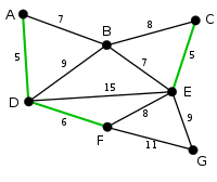
	AD and CE are the shortest edges, with length 5, and AD has been arbitrarily chosen, so it is highlighted.
	CE is now the shortest edge that does not form a cycle, with length 5, so it is highlighted as the second edge.
	The next edge, DF with length 6, is highlighted using much the same method.
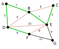
	The next-shortest edges are AB and BE, both with length 7. AB is chosen arbitrarily, and is highlighted. The edge BD has been highlighted in red, because there already exists a path (in green) between B and D, so it would form a cycle (ABD) if it were chosen.
	The process continues to highlight the next-smallest edge, BE with length 7. Many more edges are highlighted in red at this stage: BC because it would form the loop BCE, DE because it would form the loop DEBA, and FE because it would form FEBAD.
	Finally, the process finishes with the edge EG of length 9, and the minimum spanning tree is found.

Proof of correctness[]

The proof consists of two parts. First, it is proved that the algorithm produces a spanning tree. Second, it is proved that the constructed spanning tree is of minimal weight.

Spanning tree[]

Let ${\displaystyle G}$ be a connected, weighted graph and let ${\displaystyle Y}$ be the subgraph of ${\displaystyle G}$ produced by the algorithm. ${\displaystyle Y}$ cannot have a cycle, as by definition an edge is not added if it results in a cycle. ${\displaystyle Y}$ cannot be disconnected, since the first encountered edge that joins two components of ${\displaystyle Y}$ would have been added by the algorithm. Thus, ${\displaystyle Y}$ is a spanning tree of ${\displaystyle G}$.

Minimality[]

We show that the following proposition P is true by induction: If F is the set of edges chosen at any stage of the algorithm, then there is some minimum spanning tree that contains F and none of the edges rejected by the algorithm.

• Clearly P is true at the beginning, when F is empty: any minimum spanning tree will do, and there exists one because a weighted connected graph always has a minimum spanning tree.
• Now assume P is true for some non-final edge set F and let T be a minimum spanning tree that contains F.
  • If the next chosen edge e is also in T, then P is true for F + e.
  • Otherwise, if e is not in T then T + e has a cycle C. This cycle contains edges which do not belong to F, since e does not form a cycle when added to F but does in T. Let f be an edge which is in C but not in F + e. Note that f also belongs to T, and by P has not been considered by the algorithm. f must therefore have a weight at least as large as e. Then T − f + e is a tree, and it has the same or less weight as T. So T − f + e is a minimum spanning tree containing F + e and again P holds.
• Therefore, by the principle of induction, P holds when F has become a spanning tree, which is only possible if F is a minimum spanning tree itself.

Parallel algorithm[]

Kruskal's algorithm is inherently sequential and hard to parallelize. It is, however, possible to perform the initial sorting of the edges in parallel or, alternatively, to use a parallel implementation of a binary heap to extract the minimum-weight edge in every iteration.^[3] As parallel sorting is possible in time ${\displaystyle O(n)}$ on ${\displaystyle O(\log n)}$ processors,^[4] the runtime of Kruskal's algorithm can be reduced to O(E α(V)), where α again is the inverse of the single-valued Ackermann function.

A variant of Kruskal's algorithm, named Filter-Kruskal, has been described by Osipov et al.^[5] and is better suited for parallelization. The basic idea behind Filter-Kruskal is to partition the edges in a similar way to quicksort and filter out edges that connect vertices of the same tree to reduce the cost of sorting. The following pseudocode demonstrates this.

function filter_kruskal(G) is
    if |G.E| < kruskal_threshold:
        return kruskal(G)
    pivot = choose_random(G.E)
    ${\displaystyle E_{\leq }}$, ${\displaystyle E_{>}}$ = partition(G.E, pivot)
    A = filter_kruskal(${\displaystyle E_{\leq }}$)
    ${\displaystyle E_{>}}$ = filter(${\displaystyle E_{>}}$)
    A = A ∪ filter_kruskal(${\displaystyle E_{>}}$)
    return A

function partition(E, pivot) is
    ${\displaystyle E_{\leq }}$ = ∅, ${\displaystyle E_{>}}$ = ∅
    foreach (u, v) in E do
        if weight(u, v) <= pivot then
            ${\displaystyle E_{\leq }}$ = ${\displaystyle E_{\leq }}$ ∪ {(u, v)}
        else
            ${\displaystyle E_{>}}$ = ${\displaystyle E_{>}}$ ∪ {(u, v)}
    return ${\displaystyle E_{\leq }}$, ${\displaystyle E_{>}}$

function filter(E) is
    ${\displaystyle E_{\text{filtered}}}$ = ∅
    foreach (u, v) in E do
        if find_set(u) ≠ find_set(v) then
            ${\displaystyle E_{\text{filtered}}}$ = ${\displaystyle E_{\text{filtered}}}$ ∪ {(u, v)}
    return ${\displaystyle E_{\text{filtered}}}$

Filter-Kruskal lends itself better for parallelization as sorting, filtering, and partitioning can easily be performed in parallel by distributing the edges between the processors.^[5]

Finally, other variants of a parallel implementation of Kruskal's algorithm have been explored. Examples include a scheme that uses helper threads to remove edges that are definitely not part of the MST in the background,^[6] and a variant which runs the sequential algorithm on p subgraphs, then merges those subgraphs until only one, the final MST, remains.^[7]

See also[]

• Prim's algorithm
• Dijkstra's algorithm
• Borůvka's algorithm
• Reverse-delete algorithm
• Single-linkage clustering
• Greedy geometric spanner

References[]

• Thomas H. Cormen, Charles E. Leiserson, Ronald L. Rivest, and Clifford Stein. Introduction to Algorithms, Second Edition. MIT Press and McGraw-Hill, 2001. ISBN 0-262-03293-7. Section 23.2: The algorithms of Kruskal and Prim, pp. 567–574.
• Michael T. Goodrich and Roberto Tamassia. Data Structures and Algorithms in Java, Fourth Edition. John Wiley & Sons, Inc., 2006. ISBN 0-471-73884-0. Section 13.7.1: Kruskal's Algorithm, pp. 632..

External links[]

• Data for the article's example.
• Gephi Plugin For Calculating a Minimum Spanning Tree source code.
• Kruskal's Algorithm with example and program in c++
• Kruskal's Algorithm code in C++ as applied to random numbers
• Kruskal's Algorithm code in Python with explanation