LMS color space

Normalized responsivity spectra of human cone cells, S, M, and L types (SMJ data based on Stiles and Burch RGB color-matching)^[1]

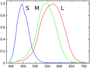
LMS (long, medium, short), is a color space which represents the response of the three types of cones of the human eye, named for their responsivity (sensitivity) peaks at long, medium, and short wavelengths.

The numerical range is generally not specified, except that the lower end is generally bounded by zero. It is common to use the LMS color space when performing chromatic adaptation (estimating the appearance of a sample under a different illuminant). It's also useful in the study of color blindness, when one or more cone types are defective.

XYZ to LMS[]

Typically, colors to be adapted chromatically will be specified in a color space other than LMS (e.g. sRGB). The chromatic adaptation matrix in the diagonal von Kries transform method, however, operates on tristimulus values in the LMS color space. Since colors in most colorspaces can be transformed to the XYZ color space, only one additional transformation matrix is required for any color space to be adapted chromatically: to transform colors from the XYZ color space to the LMS color space.^[2]

In addition, many color adaption methods, or color appearance models (CAMs), runs a von Kries-style diagonal matrix transform in a slightly modified, LMS-like, space instead. They may refer to it simply as LMS, as RGB, or as ργβ. The following text uses the "RGB" naming, but do note that the resulting space has nothing to do with the additive color model called RGB.^[2]

The CAT matrices for some CAMs in terms of CIEXYZ coordinates are presented here. The matrices, in conjunction with the XYZ data defined for the standard observer, implicitly define a "cone" response for each cell type.

Notes:

• All tristimulus values are normally calculated using the CIE 1931 2° standard colorimetric observer.^[2]
• Unless specified otherwise, the CAT matrices are normalized (the elements in a row add up to 1) so the tristimulus values for an equal-energy illuminant (X=Y=Z), like CIE Illuminant E, produce equal LMS values.^[2]

Hunt, RLAB[]

This article is missing information about how the HPE matrix was derived – looks like the most "physiological" of the XYZ bunch, but where's the data?. Please expand the article to include this information. Further details may exist on the talk page. (October 2021)

The Hunt and RLAB color appearance models use the Hunt-Pointer-Estevez transformation matrix (M_HPE) for conversion from CIE XYZ to LMS.^[3][4][5] This is the transformation matrix which was originally used in conjunction with the von Kries transform method, and is therefore also called von Kries transformation matrix (M_vonKries).

Equal-energy illuminants:	${\displaystyle {\begin{bmatrix}L\\M\\S\end{bmatrix}}_{\text{E}}={\begin{bmatrix}0.38971&0.68898&-0.07868\\-0.22981&1.18340&0.04641\\0.00000&0.00000&1.00000\end{bmatrix}}{\begin{bmatrix}X\\Y\\Z\end{bmatrix}}}$
Normalized[6] to D65:	${\displaystyle {\begin{bmatrix}L\\M\\S\end{bmatrix}}_{\text{D65}}={\begin{bmatrix}0.4002&0.7076&-0.0808\\-0.2263&1.1653&0.0457\\0&0&0.9182\end{bmatrix}}{\begin{bmatrix}X\\Y\\Z\end{bmatrix}}}$

Bradford's spectrally sharpened matrix (LLAB, CIECAM97s)[]

The original CIECAM97s color appearance model uses the Bradford transformation matrix (M_BFD) (as does the LLAB color appearance model).^[2] This is a “spectrally sharpened” transformation matrix (i.e. the L and M cone response curves are narrower and more distinct from each other). The Bradford transformation matrix was supposed to work in conjunction with a modified von Kries transform method which introduced a small non-linearity in the S (blue) channel. However, outside of CIECAM97s and LLAB this is often neglected and the Bradford transformation matrix is used in conjunction with the linear von Kries transform method, explicitly so in ICC profiles.^[7]

${\displaystyle {\begin{bmatrix}R\\G\\B\end{bmatrix}}_{\text{BFD}}={\begin{bmatrix}0.8951&0.2664&-0.1614\\-0.7502&1.7135&0.0367\\0.0389&-0.0685&1.0296\end{bmatrix}}{\begin{bmatrix}X\\Y\\Z\end{bmatrix}}}$

A "spectually sharpened" matrix is believed to improve chromatic adaptation especially for blue colors, but does not work as a real cone-describing LMS space for later human vision processing. Although the outputs are called "LMS" in its original LLAB incarceration, CIECAM97s uses a different "RGB" name to highlight that this space does not really reflect cone cells; hence the different names here.

LLAB proceeds by taking the post-adaptation XYZ values and performing a CIELAB-like treatment to get the visual correlates. On the other hand, CIECAM97s takes the post-adaptation XYZ value back into the Hunt LMS space, and works from there to model the vision system's calculation of color properties.

Later CIECAMs[]

A revised version of CIECAM97s switches back to a linear transform method and introduces a corresponding transformation matrix (M_CAT97s):^[8]

${\displaystyle {\begin{bmatrix}R\\G\\B\end{bmatrix}}_{\text{97}}={\begin{bmatrix}0.8562&0.3372&-0.1934\\-0.8360&1.8327&0.0033\\0.0357&-0.0469&1.0112\end{bmatrix}}{\begin{bmatrix}X\\Y\\Z\end{bmatrix}}}$

The sharpened transformation matrix in CIECAM02 (M_CAT02) is:^[9][2]

${\displaystyle {\begin{bmatrix}R\\G\\B\end{bmatrix}}_{\text{02}}={\begin{bmatrix}0.7328&0.4296&-0.1624\\-0.7036&1.6975&0.0061\\0.0030&0.0136&0.9834\end{bmatrix}}{\begin{bmatrix}X\\Y\\Z\end{bmatrix}}}$

CAM16 uses a different matrix:^[10]

        [+0.401288, +0.650173, -0.051461],
 M16 =  [-0.250268, +1.204414, +0.045854],
        [-0.002079, +0.048952, +0.953127].

As in CIECAM97s, after adaptation, the colors are converted to the traditional Hunt–Pointer–Estévez LMS for final prediction of visual results.

Direct from spectra[]

From a physiological point of view, the LMS color space describes a more fundamental level of human visual response, so it makes more sense to define the physiopsychological XYZ by LMS, rather than the other way around.

Stockman & Sharpe (2000)[]

A set of physiologically-based LMS functions are proposed by Stockman & Sharpe in 2000. The function has been published in a technical report by the CIE in 2006 (CIE 170).^[11] The functions are derived from Stiles and Burch (1959) RGB CMF data, combined with newer measurements about the contribution of each cone in the RGB functions. To adjust from the 10° data to 2°, assumptions about photopigment density difference and data about the absorption of light by pigment in the lens and the macula lutea are used.^[12]

The Stockman & Sharpe functions can then be turned into a set of three color-matching functions similar to those in CIEXYZ:^[13] ${\displaystyle {\begin{bmatrix}X\\Y\\Z\end{bmatrix}}_{\text{F}}={\begin{bmatrix}1.94735469&-1.41445123&0.36476327\\0.68990272&0.34832189&0\\0&0&1.93485343\end{bmatrix}}{\begin{bmatrix}L\\M\\S\end{bmatrix}}}$

The inverse matrix is shown here for comparison with the ones for traditional XYZ:

${\displaystyle {\begin{bmatrix}L\\M\\S\end{bmatrix}}={\begin{bmatrix}0.210576&0.855098&-0.0396983\\-0.417076&1.17726&0.0786283\\0&0&0.516835\\\end{bmatrix}}{\begin{bmatrix}X\\Y\\Z\end{bmatrix}}_{\text{F}}}$

Applications[]

Color blindness[]

The LMS color space can be used to emulate the way color-blind people see color. An early emulation of dichromats were produced by Brettel et al. 1997 and was rated favorably by actual patients. An example of a state-of-the-art method is Machado et al. 2009.^[14]

A related application is making color filters for color-blind people to more easily notice differences in color, a process known as daltonization.^[15]

Image processing[]

JPEG XL uses an XYB color space derived from LMS. Its transform matrix is shown here:

${\displaystyle {\begin{bmatrix}X\\Y\\B\end{bmatrix}}={\begin{bmatrix}1&-1&0\\1&1&0\\0&0&1\end{bmatrix}}{\begin{bmatrix}L\\M\\S\end{bmatrix}}}$

This can be interpreted as a hybrid color theory where L and M are opponents but S is handled in a trichromatic way, justified by the lower spatial density of S cones. In practical terms, this allows for using less data for storing blue signals without losing much perceived quality.^[16]

The colorspace originates from Guetzli's butteraugli metric,^[17] and was passed down to JPEG XL via Google's Pik project.

See also[]

• Color balance
• Color vision
• Luminosity function
• Trichromacy

References[]