Paleostress inversion
This article needs additional citations for verification. (January 2017) |
Paleostress inversion refers to the determination of paleostress history from evidence found in rocks, based on the principle that past tectonic stress should have left traces in the rocks.[1] Such relationships have been discovered from field studies for years: qualitative and quantitative analyses of deformation structures are useful for understanding the distribution and transformation of paleostress fields controlled by sequential tectonic events.[2] Deformation ranges from microscopic to regional scale, and from brittle to ductile behaviour, depending on the rheology of the rock, orientation and magnitude of the stress etc. Therefore, detailed observations in outcrops, as well as in thin sections, are important in reconstructing the paleostress trajectories.
Inversions require assumptions in order to simplify the complex geological processes. The stress field is assumed to be spatially uniform for a faulted rock mass and temporally stable over the concerned period of time when faulting occurred in that region. In other words, the effect of local fault slip is ignored in the variation in small-scale stress field. Moreover, the maximum shear stress resolved on the fault surface from the known stress field and the slip on each of the fault surface has the same direction and magnitude.[3] Since the first introduction of the methods by Wallace[4] and Bott[5] in the 1950s, similar assumptions have been used throughout the decades.
Fault slip analysis[]
Conjugate fault system[]
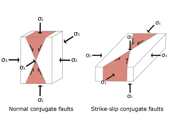
Anderson[6][7] was the first to utilize conjugate fault systems in interpreting paleostress, including all kinds of conjugate faults (normal, reverse and strike-slip). Regional conjugate fault can be better understood by comparison to a familiar rock mechanics experiment, i.e. the Uniaxial Compressive Strength (UCS) Test. Basics of their mechanisms are similar except the principal stress orientation applied is rotated from perpendicular to parallel to the ground. The conjugate fault model is a simple way to obtain approximate orientations of stress axes, due to the abundance of such structure in the upper brittle crust. Therefore, a number of studies have been carried out by other researchers in assorted structural settings and by correlating with other deformation structures.[8]
Nonetheless, further development revealed the deficiency of the model:
- 1. Important geometrical properties absent in practical situation
The geometrical properties of conjugate faults are indicative of the sense of stress, but they may not appear in the actual fault patterns.
- Slickenside lineations normal to fault plane intersection
- Symmetrical sense of motion that gives the obtuse angle in the direction of lengthening
- Relation between the intersecting angle of fault planes and mechanical properties, with reference to information from rock mechanics experiments in lab
- 2. Observed fault patterns are far more sophisticated
There are often oblique pre-existing faults, planes of weaknesses or striations to the fault slip, which do not belong to the conjugate fault sets. Neglecting this considerable amount of data would cause error in analysis.
- 3. Neglecting the stress ratio (Φ)
This ratio provides the relative magnitude of the intermediate stress (σ2) and thus determines the shape of the stress ellipsoid. However, this model does not give an account on the ratio, save for some specific cases.
Reduced stress tensor[]
This method was established by Bott[5] in 1959, based on the assumption that direction and sense of slip occurs on the fault plane are the same with those of the maximum resolved shear stress, hence, with known orientations and senses of movements on abundant faults, a particular solution T (the reduce stress tensor) is attained.[5] It gives more comprehensive and accurate results in reconstructing paleostress axes and determining the stress ratio (Φ) than the conjugate fault system. The tensor works by solving for four independent unknowns (three principal axes and Φ) through mathematical computation of observations of faults (i.e. attitude of faults and lineations on fault planes, direction and sense of slip, and other tension fractures).
This method follows four rigorous steps:
- Data Analysis
- Computation of Reduced Stress Tensor
- Minimization
- Check of Results
Data analysis[]
Reconstruction of paleostress requires large amount of data to attain accuracy, so it is essential to organize the data in comprehensible format prior to any analysis.

- 1) Fault Population Geometry
Attitude of fault planes and slickensides is plotted on rose diagrams, such that the geometry is visible. This is particularly useful when the sample size is enormous, it provides the full picture of the region of interest.

- 2) Fault Motion
Fault movement is resolved into three components (as in 3D), which are vertical transverse, horizontal transverse and lateral components, by trigonometric relation with the measured dips and trends. Net slip is shown more clearly which paves the way to understanding the deformation.

- 3) Individual Fault Geometry
Fault planes are represented by lines in stereonets (equal area lower hemisphere projection), while rakes on them are indicated by dots sitting on the lines. It helps to visualize the geometrical distribution and possible symmetry among individual faults.
- 4) P (pressure) and T (tension) Dihedra[9]
This is a concluding step of compiling all the data and check their mechanical compatibility, also could be seen a preliminary step in determining major paleostress orientations. As this is a simple graphical representation of the fault geometry (being the boundaries of dihedra) and sense of slip (shortening direction indicated by black and extension depicted by grey), while it is able to provide good constraints on the orientation of principal stress axes.
The approximation is built upon the assumption that the orientation of maximum principal stress (σ1) most probably passes through the greatest number of P-quadrants. Since fault plane and auxiliary plane perpendicular to striations are considered the same in this method, the model can be directly applied to focal mechanisms of earthquakes. Nonetheless, due to the same reason, this method cannot provide accurate determination of paleostress, as well as the stress ratio.

- 4) Principle of P and T dihedra: incompatibility zones (white) are found by overlapping P (black) and T (grey) regions derived from fault sets
Determination of paleostress[]
Reduced stress tensor[]
Stress tensor can be considered as a matrix with nine components being the nine stress vectors acting on a point, in which the three vectors along the diagonal (highlighted in brown) represent the principal axes.

The reduced stress tensor is a mathematical computation approach to determining the three principal axes and the stress ratio, totally four independent unknowns, calculated as eigenvectors and eigenvalue respectively, so that this method is more complete and accurate than the mentioned graphical approaches.

There are a number formulations that can reach the same final results but with distinctive features:
(1) ,

where , such that .[10] This tensor is defined by setting σ1, σ2 and σ3 as 1, Φ and 0 (highlighted in pink) respectively, due to choosing and as the mode of reduction. The advantage of this formulation is the direct correspondence to stress orientation, thus the stress ellipsoid, and the stress ratio.


(2)

This formulation is a deviator, which requires more computation to obtain information of the stress ellipsoid despite maintaining a symmetry in mathematical context.[11]
Minimization[]
Minimization aims to reduce the differences between the computed and observed slip directions of fault planes by choosing a function to proceed the least square minimization. Here are a few examples of the functions:
| sum of terms | |
| unit pole (normal) to fault plane | |
| unit slip vector | |
| applied stress vector | |
| shear stress |


(1)

The very first function used in fault slip analysis does not account on the sense of individual slip, which means altering the sense of a single slip does not affect the result.[12] However, individual sense of motion is an effective reflection of orientation of stress axes in real situation. Hence, S1 is the simplest function but include the importance of sense of individual slip.
(2)

S2 is derived from S1 based on variation in computational process.
(3)
![{\displaystyle S_{3}=\sum \min[\tan ^{2}({\vec {s}}_{k},{\vec {\tau }}_{k})^{2},1]}](https://wikimedia.org/api/rest_v1/media/math/render/svg/252542c0df6cdc7b5e7f267cf07ebb9dde5faaa6)
S3 is an improved version of the previous model in two aspects. Regarding the efficiency in computation, which is particularly significant in long iterative processes like this, tangent of angles is preferred to cosine. Moreover, to deal with anomalous data (e.g. faults initiated by another event, error in data collection etc.), an upper limit of the value of the functions of angle could be set to filter deviated data.
(4)

S4 resembles S2 except the unit vector parallel to shear stress is substituted by the predicted shear stress. Therefore, it still produces similar results as other methods, although its physical meaning is less well justified.
Checking results[]
The reduced stress tensor should best (hardly perfectly) describe the observed orientations and senses of movement on diversified fault planes in a rock mass. Therefore, by reviewing the fundamental principle of interpreting paleostress from the reduced stress tensor, an assumption is recognized: every fault slip in the rock mass is induced homogeneously by a common stress tensor. This implies the variation in stress orientation and ratio Φ within a rock mass is overlooked yet always present in practical case, due to interaction between discontinuities at any scale.
Hence, the significance of this effect has to be examined to test the validity of the method, by considering the parameter: the difference between the measured slickenside lineation and the theoretical shear stress. The average angular deviation is insignificant when compared with the total of instrumental (measuring tools) and observation (unevenness of fault surfaces and striae) errors in majority of the cases.[11]
In conclusion, the reduced stress tensor method is validated when
- sample size is large and representative (homogeneous data sets with a range of fault orientations),
- sense of motion of is noted,
- minimization of angular difference is emphasized when choosing functions (mentioned in section above), and
- rigorous computation takes place.
Limitation[]
Quantitative analyses cannot stand alone without careful qualitative field observations. The above described analyses are to be carried out after the overall geologic framework is understood e.g. number of paleostress systems, chronological order of successive stress patterns. Also, consistency with other stress markers e.g. stylolites and tension fractures, is required to justify the result.
Examples of application[]
- Cambrian Eriboll Formation sandstones west of the Moine Thrust Zone, NW Scotland[13]
- Baikal region, Central Asia[14]
- Alpine foreland, Central Northern Switzerland[15]
Grain boundary piezometer[]
A piezometer is an instrument used in the measurement of pressure (non-directional) or stress (directional) from strain in rocks at any scale. Referring to the paleostress inversion principle, rock masses under stress should exhibit strain at both macroscopic and microscopic scale, while the latter is found at the grain boundaries (interface between crystal grains at the magnitude below 102μm). Strain is revealed from the change in grain size, orientation of grains or migration of crystal defects, through a number of mechanisms e.g. dynamic recrystallization (DRX).
Since these mechanisms primarily depend on flow stress and their resulted deformation is stable, the strained grain size or grain boundary are often used as an indicator of paleostress in tectonically active regions such as crustal shear zones, orogenic belts and the upper mantle.[16]
Dynamic recrystallization (DRX)[]
Dynamic recrystallization is one of the crucial mechanisms in reducing grain size in shear setting.[17] DRX is defined as a nucleation-and-growth process because
- local grain boundary bulging (BLG) (mechanisms of nucleation)
- subgrain rotation (SGR) (mechanisms of nucleation)
- grain boundary migration (GBM) (mechanisms of grain growth),
are all present in the deformation. This evidence is commonly found in quartz, a typical piezometer, from ductile shear zones. Optical microscope and transmission electron microscope (TEM) are usually utilized in observing the sequential occurrence of subgrain rotation and local grain boundary bulging, and measuring recrystallized grain size. The nucleation process is triggered at boundaries of existing grains only when materials have been deformed to particular critical values.
Grain boundary bulging (BLG)[]

Grain boundary bulging is the process involving the growth of nuclei at the expense of existing grains and then formation of a 'necklace' structure.

Subgrain rotation (SGR)[]
Subgrain rotation is also known as in-situ recrystallization without considerable grain growth. This process happens steadily over the strain history, thus the change in orientation is progressive but not abrupt as grain boundary bulging.
Therefore, grain boundary bulging and subgrain rotation are differentiated as discontinuous and continuous dynamic recrystallization respectively.
Theoretical models[]
Static energy-balance model[]
The theoretical basis of grain size piezometry was first established by Robert J. Twiss in late 1970s.[18] By comparing free dislocation energy and grain boundary energy, he derived a static energy balance model applicable to subgrain size . Such relation has been represented by an empirical equation between normalized value of grain size and flow stress, which is universal for various materials:
- ,

d is the average grain size;
b is the length of the Burgers vector;
K is a non-dimensional temperature-dependent constant, which is typically in the order of 10;
μ is the shear modulus;
σ is the flow stress.
This model does not account for the persistently transforming nature of microstructures seen in dynamic recrystallization, so its inability in determination of recrystallized grain size has led to the latter models.
Nucleation-and-growth models[]
Unlike the previous model, these models consider the sizes of individual grains vary temporally and spatially, therefore, they derive an average grain size from an equilibrium between nucleation and grain growth. The scaling relation of the grain size is as follows:
- ,

where d is the mode of logarithmic grain size, I is the nucleation rate per unit volume, and a is a scaling factor. Upon this basic theory, there are still plenty of arguments on the details, which are reflected in the assumptions of the models, so there are various modifications.
- Derby–Ashby model[19]
Derby and Ashby considered boundary bulging nucleation at grain boundary in determining the nucleation rate (Igb), which opposes to the intracrystalline nucleation suggested by the prior model. Thus this model describes the microstructures of discontinuous DRX (DDRX):
- .

- Shimizu model[20]
Because of a contrasting assumption that subgrain rotation nucleation in continuous DRX (CDRX) should be considered for the nucleation rate, Shimizu has come up with another model, which has also been tested in laboratory:
- .

Simultaneous operation of dislocation and diffusion creeps[]
Field boundary model[21]
In the above models, one of the vital factors, especially when the grain size is reduced substantially through dynamic recrystallization, is neglected. The surface energy becomes more significant when grains are sufficiently small, which converts the creep mechanism from dislocation creep to diffusion creep, thus the grains start to grow. Therefore, the determination of the boundary zone between fields of these two creep mechanisms matter to know when the recrystallized grain size tends to stabilize, as to supplement the above model.[21] The difference between this model and the previous nucleation-and-growth models lies within the assumptions: the field boundary model assumes that grain size reduces in the dislocation creep field, and enlarges in the diffusion creep field, but it is not the case in the previous models.
Common piezometers[]
Quartz is abundant in the crust and contains creep microstructures that are sensitive to deformation conditions in deeper crust. Before starting to infer flow stress magnitude, the mineral has to be calibrated carefully in laboratory. Quartz has been found to exhibit different piezometer relations during different recrystallization mechanisms, which are local grain boundary migration (dislocation creep), (SGR) and the combination of these two, as well as at different grain size.[22]
Other common minerals used for grain size piezometers are calcite and halite, that have gone through syn-tectonic deformation or manual high-temperature creep, which also demonstrate difference in piezometer relation for distinct recrystallization mechanisms.[22]
Further reading[]
- Angelier, J., 1994, Fault slip analysis and paleostress reconstruction. In: Hancock, P.L. (ed.), Continental Deformation. Pergamon, Oxford, p. 101–120.
- Célérier, B., Etchecopar, A., Bergerat, F., Vergely, P., Arthaud, F., Laurent, P., 2012. Inferring stress from faulting: From early concepts to inverse methods. Tectonophysics, Crustal Stresses, Fractures, and Fault Zones: The Legacy of Jacques Angelier 581, 206–219.
- Pascal, C., 2021. Paleostress Inversion Techniques: Methods and Applications for Tectonics, Elsevier, 400 p. https://www.elsevier.com/books/paleostress-inversion-techniques/pascal/978-0-12-811910-5
- Ramsay, J.G., Lisle, R.J., 2000. The Techniques of Modern Structural Geology. Volume 3: Applications of continuum mechanics in structural geology (Session 32: Fault Slip Analysis and Stress Tensor Calculations), Academic Press, London.
- Yamaji, A., 2007. An Introduction to Tectonophysics: Theoretical Aspects of Structural Geology (Chapter 11: Determination of Stress from Faults), Terrapub, Tokyo. http://www.terrapub.co.jp/e-library/yamaji/
References[]
- ^ Angelier, J., 1994, Fault slip analysis and paleostress reconstruction. In: Hancock, P.L. (ed.), Continental Deformation. Pergamon, Oxford, p. 101–120.
- ^ Angelier, J. (1989). From orientation to magnitudes in paleostress determinations using fault slip data. Journal of Structural Geology. Vol. 11 No. 1/2. pp37-50
- ^ J. O. Kaven et al. (2011). Mechanical analysis of fault slip data: Implications for paleostress analysis. Journal of Structural Geology. Vol. 33. pp78-91.
- ^ Wallace, R. E. 1951. Geometry of shearing stress and relation to faulting. J. Geol. 59, 118-130.
- ^ a b c Bott, M. H. P. 1959. The mechanisms of oblique slip faulting. Geol. Mag. 96,109-117.
- ^ Anderson, E.M., 1905. The dynamics of faulting. Transactions of the Edinburgh Geological Society 8, 387–402.
- ^ Anderson, E. M. 1942. The Dynamics of Faulting. Oliver and Boyd, Edinburgh, 1st ed, 206.
- ^ Arthaud, F. and Mattauer M. 1969. Exemple de Stylolites d'origine tectonique dans le Languedoc, leurs relations avec la tectonique cassante. Bull. Soc. Geol. Fr., XI (7), 738-744.
- ^ Angelier, J. and Mechler, P. 1977. Sur une methode graphique de recherche des contraintes principles egalement utilisable en tectonique et en seismologie: la methode des diedres droits. Bull. Soc. geol. Fr. 19, 1309-1318.
- ^ Angelier, J. 1975. Sur l'analyse de mesures recueillies dam des sites failles: L'utilite d'une confrontation entre les methodes dynamiques et cinematiques. C.r. Acad. Sci., Paris D281, 1805-1808.
- ^ a b Angelier, J. 1984. Tectonic Analysis of Fault Slip Data Sets. Journal of Geophysical Research, 89, B7, 5835-5848.
- ^ Angelier, J. 1979b. Determination of the mean principal directions of stresses for a given fault population. Tectonophysics, 56, 17-26.
- ^ Laubach, S. E. and Diaz-Tushman, K. 2009. Laurentian palaeostress trajectories and ephemeral fracture permeability, Cambrian Eriboll Formation sandstones west of the Moine Thrust Zone, NW Scotland. Journal of the Geological Society, London, Vol. 166, 349–362.
- ^ Delvaux et al. 1995. Paleostress reconstructions and geodynamics of the Baikal region, Central Asia, Part I. Palaeozoic and Mesozoic pre-rift. Tectonophysics 252, 61- 101.
- ^ Madritsch, H. 2015. Outcrop-scale fracture systems in the Alpine foreland of central northern Switzerland: kinematics and tectonic context. Swiss J Geosci 108, 155–181.
- ^ Shimizu, I. 2008. Theories and applicability of grain size piezometers: The role of dynamic recrystallization mechanisms. Journal of Structural Geology. Vol. 30. pp899-917
- ^ Tullis, J., Yund, R.A., 1985. Dynamic recrystallization of feldspar: a mechanism for ductile shear zone formation. Geology 13, 238–241.
- ^ Twiss, R. J. 1977. Theory and Applicability of a Recrystallized Grain Size Paleopiezometer. Pageoph, 115. Birkhauser: Basel.
- ^ Derby, B., Ashby, M.F., 1987. On dynamic recrystallization. Scripta Metallurgica 21, 879–884
- ^ Shimizu, I., 1998b. Stress and temperature dependence of recrystallized grain size: a subgrain misorientation model. Geophysical Research Letters 25, 4237–4240.
- ^ a b De Bresser, J.H.P., Peach, C.J., Reijs, J.P.J., Spiers, C.J., 1998. On dynamic recrystallization during solid state flow: effects of stress and temperature. Geophysical Research Letters 25, 3457–3460.
- ^ a b Stipp M. and Tullis Jan. 2003. The recrystallized grain size piezometer for quartz. Geophysical Research Letters. Vol. 30, 21.
- Structural geology
- Deformation (mechanics)