Profit maximization
In economics, profit maximization is the short run or long run process by which a firm may determine the price, input and output levels that lead to the highest profit. Neoclassical economics, currently the mainstream approach to microeconomics, usually models the firm as maximizing profit.
An example diagram of Profit Maximisation:

In the supply and demand graph, the output of Q* is the intersection point of MR and MC. The firm produces at this output level can maximize profits. (MR=MC) When produced less than Output of equilibrium quantity (Q*), as the red part showed, MR is greater than MC. The firm produce extra output because the revenue of gaining is more than the cost to pay. So, total profit will increase. However, if the output level is greater than Q*, MR<MC as the blue part showed. The firm profit will decrease because the extra unit level increase the cost which is greater than the revenue. So, total profit will decrease.
There are several perspectives one can take on profit maximization . First, since profit equals revenue minus cost, one can plot graphically each of the variables revenue and cost as functions of the level of output and find the output level that maximizes the difference (or this can be done with a table of values instead of a graph). Second, if specific functional forms are known for revenue and cost in terms of output, one can use calculus to maximize profit with respect to the output level. Third, since the first order condition for the optimization equates marginal revenue and marginal cost, if marginal revenue (mr) and marginal cost(mc) functions in terms of output are directly available one can equate these, using either equations or a graph. Fourth, rather than a function giving the cost of producing each potential output level, the firm may have input cost functions giving the cost of acquiring any amount of each input, along with a production function showing how much output results from using any combination of input quantities. In this case one can use calculus to maximize profit with respect to input usage levels, subject to the input cost functions and the production function. The first order condition for each input equates the marginal revenue product of the input (the increment to revenue from selling the product caused by an increment to the amount of the input used) to the marginal cost of the input.
For a firm in a perfectly competitive market for its output, the revenue function will simply equal the market price times the quantity produced and sold, whereas for a monopolist, which chooses its level of output simultaneously with its selling price. In the case of monopoly, the company will produce more products because it can still make normal profits. To get the most profit, you need to set higher prices and lower quantities than the competitive market. However, the revenue function takes into account the fact that higher levels of output require a lower price in order to be sold. An analogous feature holds for the input markets: in a perfectly competitive input market the firm's cost of the input is simply the amount purchased for use in production times the market-determined unit input cost, whereas a monopsonist’s input price per unit is higher for higher amounts of the input purchased.
The principal difference between short-run and long-run profit maximization is that in the long run the quantities of all inputs, including physical capital, are choice variables, while in the short run the amount of capital is predetermined by past investment decisions. In either case there are inputs of labor and raw materials.
Limitations of profit maximization The limitations of the concept of profit maximization are low, and any behavior will not only bring a certain level of profit. On the contrary, there can produce many different profit levels, and each profit level can happen.
Basic definitions[]
Any costs incurred by a firm may be classed into two groups: fixed costs and variable costs. Fixed costs, which occur only in the short run, are incurred by the business at any level of output, including zero output. These may include equipment maintenance, rent, wages of employees whose numbers cannot be increased or decreased in the short run, and general upkeep. Variable costs change with the level of output, increasing as more product is generated. Materials consumed during production often have the largest impact on this category, which also includes the wages of employees who can be hired and laid off in the short-run span of time under consideration. Fixed cost and variable cost, combined, equal total cost.
Revenue is the amount of money that a company receives from its normal business activities, usually from the sale of goods and services (as opposed to monies from security sales such as equity shares or debt issuances).
The five ways formula is to increase leads, conversation rates, average dollar sale, average number of sales and average product profit. Profits can be increased by up to 1000 percent, this is important for sole traders and small businesses let alone big businesses but none the less all profit maximization is a matter of each business stage and greater returns for profit sharing thus higher wages and motivation.[1]
Marginal cost and marginal revenue, depending on whether the calculus approach is taken or not, are defined as either the change in cost or revenue as each additional unit is produced, or the derivative of cost or revenue with respect to the quantity of output. For instance, taking the first definition, if it costs a firm $400 to produce 5 units and $480 to produce 6, the marginal cost of the sixth unit is 80 dollars. Conversely, the marginal income from the production of 6 units is the income from the production of 6 units minus the income from the production of 5 units (the latter item minus the preceding item).
Total revenue–total cost perspective[]
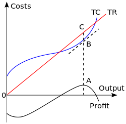
To obtain the profit maximizing output quantity, we start by recognizing that profit is equal to total revenue (TR) minus total cost (TC). Given a table of costs and revenues at each quantity, we can either compute equations or plot the data directly on a graph. The profit-maximizing output is the one at which this difference reaches its maximum.
In the accompanying diagram, the linear total revenue curve represents the case in which the firm is a perfect competitor in the goods market, and thus cannot set its own selling price. The profit-maximizing output level is represented as the one at which total revenue is the height of C and total cost is the height of B; the maximal profit is measured as the length of the segment CB. This output level is also the one at which the total profit curve is at its maximum.
If, contrary to what is assumed in the graph, the firm is not a perfect competitor in the output market, the price to sell the product at can be read off the demand curve at the firm's . This optimal quantity of output is the quantity at which marginal revenue equals marginal cost.
Marginal revenue–marginal cost perspective[]


An equivalent perspective relies on the relationship that, for each unit sold, marginal profit (Mπ) equals marginal revenue (MR) minus marginal cost (MC). Then, if marginal revenue is greater than marginal cost at some level of output, marginal profit is positive and thus a greater quantity should be produced, and if marginal revenue is less than marginal cost, marginal profit is negative and a lesser quantity should be produced. At the output level at which marginal revenue equals marginal cost, marginal profit is zero and this quantity is the one that maximizes profit.[2] Since total profit increases when marginal profit is positive and total profit decreases when marginal profit is negative, it must reach a maximum where marginal profit is zero—where marginal cost equals marginal revenue—and where lower or higher output levels give lower profit levels.[2] In calculus terms, the requirement that the optimal output have higher profit than adjacent output levels is that:[2]

The intersection of MR and MC is shown in the next diagram as point A. If the industry is perfectly competitive (as is assumed in the diagram), the firm faces a demand curve (D) that is identical to its marginal revenue curve (MR), and this is a horizontal line at a price determined by industry supply and demand. Average total costs are represented by curve ATC. Total economic profit is represented by the area of the rectangle PABC. The optimum quantity (Q) is the same as the optimum quantity in the first diagram.
If the firm is a monopolist, the marginal revenue curve would have a negative slope as shown in the next graph, because it would be based on the downward-sloping market demand curve. The optimal output, shown in the graph as Qm, is the level of output at which marginal cost equals marginal revenue. The price that induces that quantity of output is the height of the demand curve at that quantity (denoted Pm).
In an environment that is competitive but not perfectly so, more complicated profit maximization solutions involve the use of game theory.
Case in which maximizing revenue is equivalent[]
In some cases a firm's demand and cost conditions are such that marginal profits are greater than zero for all levels of production up to a certain maximum.[3] In this case marginal profit plunges to zero immediately after that maximum is reached; hence the Mπ = 0 rule implies that output should be produced at the maximum level, which also happens to be the level that maximizes revenue.[3] In other words, the profit maximizing quantity and price can be determined by setting marginal revenue equal to zero, which occurs at the maximal level of output. Marginal revenue equals zero when the total revenue curve has reached its maximum value. An example would be a scheduled airline flight. The marginal costs of flying one more passenger on the flight are negligible until all the seats are filled. The airline would maximize profit by filling all the seats.
Maximizing profits in the real world[]
In the real world, it is not easy to achieve profit maximization. The company must accurately know the marginal income and the marginal cost of the last commodity sold because of MR. The price elasticity of demand for goods depends on the response of other companies. When it is the only company raising prices, demand will be elastic. If one family raises prices and others follow, demand may be inelastic. However, companies can seek to maximize profits through estimation. When the price increase leads to a small decline in demand, the company can increase the price as much as possible before the demand becomes elastic. Generally, it is difficult to change the impact of the price according to the demand, because the demand may occur due to many other factors besides the price. Variety. The company may also have other goals and considerations. For example, companies may choose to earn less than the maximum profit in pursuit of higher market share. Because price increases maximize profits in the short term, they will attract more companies to enter the market. Habitually record and analyze the business costs of all your products/services sold. When you can know all the costs of each successful sale, accurate costs are conducive to profit analysis. However, there are many miscellaneous items in the cost including labor, materials, transportation, advertising, storage, etc. These miscellaneous items often become small expenses of the enterprise and are related to any goods or services sold.
Business intelligence tools may be needed to integrate all financial information to record expense reports, so that the business can clearly understand all costs related to operations and their accuracy Check monthly or quarterly, write down any changes and their reasons, or if possible, record problems and vulnerabilities for improvement. This information can help you improve business optimization and thereby increase profits. Forecasting demand to optimize sales, many large companies will minimize costs by shifting production to foreign locations with cheap labor (e.g. NIKE). However, moving the production line to a foreign location may cause unnecessary transportation costs. On the other hand, close market locations for producing and selling products can improve demand optimization, but when the production cost is much higher, it is not a good choice. Carry out operation management forecasts and use sales data to predict demand increase, stagnation or decline, in order to increase or decrease the production of a specific product series. Use standardized demand optimization functions to enhance the demand planning process to determine the direction of the organization's needs to maximize profits. Planning and actual execution, when implementing a "what if" solution to help you in the sales and operation planning process, you need to be familiar with the company's operations, including the supply chain, inventory management and sales process. Use constraints to prevent corporate plans from becoming unfeasible. Use the above information to better predict possible solutions for financial and supply chain management plans.
Changes in total costs and profit maximization[]
A firm maximizes profit by operating where marginal revenue equals marginal cost. In the short run, a change in fixed costs has no effect on the profit maximizing output or price.[4] The firm merely treats short term fixed costs as sunk costs and continues to operate as before.[5] This can be confirmed graphically. Using the diagram illustrating the total cost–total revenue perspective, the firm maximizes profit at the point where the slopes of the total cost line and total revenue line are equal.[3] An increase in fixed cost would cause the total cost curve to shift up rigidly by the amount of the change.[3] There would be no effect on the total revenue curve or the shape of the total cost curve. Consequently, the profit maximizing output would remain the same. This point can also be illustrated using the diagram for the marginal revenue–marginal cost perspective. A change in fixed cost would have no effect on the position or shape of these curves.[3] In simple terms, although profit is related to total cost, Profit = TR-TC, the enterprise can maximize profit by producing to the maximum profit (the maximum value of TR-TC) to maximize profit. But when the total cost increases, it does not mean maximizing profit Will change, because the increase in total cost does not necessarily change the marginal cost. If the marginal cost remains the same, the enterprise can still produce to the unit of (MR=MC=Price) to maximize profit.
Markup pricing[]
In addition to using methods to determine a firm's optimal level of output, a firm that is not perfectly competitive can equivalently set price to maximize profit (since setting price along a given demand curve involves picking a preferred point on that curve, which is equivalent to picking a preferred quantity to produce and sell). The profit maximization conditions can be expressed in a "more easily applicable" form or rule of thumb than the above perspectives use.[6] The first step is to rewrite the expression for marginal revenue as

, where P and Q refer to the midpoints between the old and new values of price and quantity respectively.[6] The marginal revenue from an incremental unit of output has two parts: first, the revenue the firm gains from selling the additional units or, giving the term P∆Q. The additional units are called the marginal units.[7] Producing one extra unit and selling it at price P brings in revenue of P. Moreover, one must consider "the revenue the firm loses on the units it could have sold at the higher price"[7]—that is, if the price of all units had not been pulled down by the effort to sell more units. These units that have lost revenue are called the infra-marginal units.[7] That is, selling the extra unit results in a small drop in price which reduces the revenue for all units sold by the amount Q(∆P/∆Q). Thus MR = P + Q(∆P/∆Q) = P +P (Q/P)(∆P/∆Q) = P + P/(PED), where PED is the price elasticity of demand characterizing the demand curve of the firms' customers, which is negative. Then setting MC = MR gives MC = P + P/PED so (P − MC)/P = −1/PED and P = MC/[1 + (1/PED)]. Thus the optimal markup rule is:
- (P − MC)/P = 1/ (−PED)
- or equivalently
In other words, the rule is that the size of the markup of price over the marginal cost is inversely related to the absolute value of the price elasticity of demand for the good.[8]
The optimal markup rule also implies that a non-competitive firm will produce on the elastic region of its market demand curve. Marginal cost is positive. The term PED/(1+PED) would be positive so P>0 only if PED is between −1 and −∞ (that is, if demand is elastic at that level of output).[10] The intuition behind this result is that, if demand is inelastic at some value Q1 then a decrease in Q would increase P more than proportionately, thereby increasing revenue PQ; since lower Q would also lead to lower total cost, profit would go up due to the combination of increased revenue and decreased cost. Thus Q1 does not give the highest possible profit.
Marginal product of labor, marginal revenue product of labor, and profit maximization[]
The general rule is that the firm maximizes profit by producing that quantity of output where marginal revenue equals marginal cost. The profit maximization issue can also be approached from the input side. That is, what is the profit maximizing usage of the variable input? [11] To maximize profit the firm should increase usage of the input "up to the point where the input's marginal revenue product equals its marginal costs".[12] So mathematically the profit maximizing rule is MRPL = MCL, where the subscript L refers to the commonly assumed variable input, labor. The marginal revenue product is the change in total revenue per unit change in the variable input. That is MRPL = ∆TR/∆L. MRPL is the product of marginal revenue and the marginal product of labor or MRPL = MR x MPL.
Sub-optimal Profit maximization[]
Oftentimes, businesses will attempt to maximize their profits even though their optimization strategy typically leads to a sub-optimal quantity of goods produced for the consumers. When deciding a given quantity to produce, a firm will often try to maximize its own producer surplus, at the expense of decreasing the overall social surplus. As a result of this decrease in social surplus, consumer surplus is also minimized, as compared to if the firm did not elect to maximize their own producer surplus.
Government Regulation[]
Market quotas reflect the power of a firm in the market, a firm dominating a market is very common, and too much power often becomes the motive for non-Hong behavior. predatory pricing, tying, price gouging and other behaviors are reflecting the crisis of excessive power of monopolists in the market. In an attempt to prevent businesses from abusing their power to maximize their own profits, governments often intervene to stop them in their tracks. A major example of this is through anti-trust regulation which effectively outlaws most industry monopolies. Through this regulation, consumers enjoy a better relationship with the companies that serve them, even though the company itself may suffer, financially speaking.
See also[]
- Business organization
- Corporation
- Duality (optimization)
- Market structure
- Microeconomics
- Pricing
- Outline of industrial organization
- Rational choice theory
- Supply and demand
- Marginal revenue
- Total revenue
- Marginal cost
Notes[]
- ^ entrepreneur.com
- ^ Jump up to: a b c Lipsey (1975). pp. 245–47.
- ^ Jump up to: a b c d e Samuelson, W and Marks, S (2003). p. 47.
- ^ Samuelson, W and Marks, S (2003). p. 52.
- ^ Landsburg, S (2002).
- ^ Jump up to: a b Pindyck, R and Rubinfeld, D (2001) p. 333.
- ^ Jump up to: a b c Besanko, D. and Beautigam, R, (2001) p. 408.
- ^ Jump up to: a b Samuelson, W and Marks, S (2003). p. 103–05.
- ^ Pindyck, R and Rubinfeld, D (2001) p. 341.
- ^ Besanko and Braeutigam (2005) p. 419.
- ^ Samuelson, W and Marks, S (2003). p. 230.
- ^ Samuelson, W and Marks, S (2003). p. 23.
References[]
- Landsg, S (2002). Price Theory and Applications (fifth ed.). South-Western.
- Lipsey, Richard G. (1975). An introduction to positive economics (fourth ed.). Weidenfeld and Nicolson. pp. 214–7. ISBN 0-297-76899-9.
- Samuelson, W; Marks, S (2003). Managerial Economics (fourth ed.). Wiley.
External links[]
- Profit Maximization in Perfect Competition by Fiona Maclachlan, Wolfram Demonstrations Project.
- Profit Maximization: The Comprehensive Guide by Richard Gulle, .
Profit Maximisation by Tejvan Pettinger. [https://www.riverlogic.com/blog/three-steps-to-mastering-profit-maximization/ Three Steps to Mastering Prescriptive Profit Maximization} by Riverlogic.
| hide Authority control | |
|---|---|
| General | |
| National libraries | |
| Other | |
- Profit
- Pricing
- Financial management