Quantum Fourier transform

In quantum computing, the quantum Fourier transform (QFT) is a linear transformation on quantum bits, and is the quantum analogue of the inverse discrete Fourier transform. The quantum Fourier transform is a part of many quantum algorithms, notably Shor's algorithm for factoring and computing the discrete logarithm, the quantum phase estimation algorithm for estimating the eigenvalues of a unitary operator, and algorithms for the hidden subgroup problem. The quantum Fourier transform was discovered by Don Coppersmith.^[1]

The quantum Fourier transform can be performed efficiently on a quantum computer, with a particular decomposition into a product of simpler unitary matrices. Using a simple decomposition, the discrete Fourier transform on ${\displaystyle 2^{n}}$ amplitudes can be implemented as a quantum circuit consisting of only ${\displaystyle O(n^{2})}$ Hadamard gates and controlled phase shift gates, where ${\displaystyle n}$ is the number of qubits.^[2] This can be compared with the classical discrete Fourier transform, which takes ${\displaystyle O(n2^{n})}$ gates (where ${\displaystyle n}$ is the number of bits), which is exponentially more than ${\displaystyle O(n^{2})}$. However, the quantum Fourier transform acts on a quantum state, whereas the classical Fourier transform acts on a vector, so not every task that uses the classical Fourier transform can take advantage of this exponential speedup.^{[citation needed]}

The best quantum Fourier transform algorithms known (as of late 2000) require only ${\displaystyle O(n\log n)}$ gates to achieve an efficient approximation.^[3]

Definition[]

The quantum Fourier transform is the classical discrete Fourier transform applied to the vector of amplitudes of a quantum state, where we usually consider vectors of length ${\displaystyle N=2^{n}}$.

The classical Fourier transform acts on a vector ${\displaystyle (x_{0},x_{1},\ldots ,x_{N-1})\in \mathbb {C} ^{N}}$ and maps it to the vector ${\displaystyle (y_{0},y_{1},\ldots ,y_{N-1})\in \mathbb {C} ^{N}}$ according to the formula:

${\displaystyle y_{k}={\frac {1}{\sqrt {N}}}\sum _{n=0}^{N-1}x_{n}\omega _{N}^{-kn},\quad k=0,1,2,\ldots ,N-1,}$

where ${\displaystyle \omega _{N}=e^{\frac {2\pi i}{N}}}$ and ${\displaystyle \omega _{N}^{n}}$ is an N^th root of unity.

Similarly, the quantum Fourier transform acts on a quantum state ${\displaystyle |x\rangle =\sum _{i=0}^{N-1}x_{i}|i\rangle }$ and maps it to a quantum state ${\displaystyle \sum _{i=0}^{N-1}y_{i}|i\rangle }$ according to the formula:

${\displaystyle y_{k}={\frac {1}{\sqrt {N}}}\sum _{n=0}^{N-1}x_{n}\omega _{N}^{nk},\quad k=0,1,2,\ldots ,N-1,}$

(Conventions for the sign of the phase factor exponent vary; here we use the convention that the quantum Fourier transform has the same effect as the inverse discrete Fourier transform, and vice versa.)

Since ${\displaystyle \omega _{N}^{n}}$ is a rotation, the inverse quantum Fourier transform acts similarly but with:

${\displaystyle x_{n}={\frac {1}{\sqrt {N}}}\sum _{k=0}^{N-1}y_{k}\omega _{N}^{-nk},\quad n=0,1,2,\ldots ,N-1,}$

In case that ${\displaystyle |x\rangle }$ is a basis state, the quantum Fourier Transform can also be expressed as the map

${\displaystyle {\text{QFT}}:|x\rangle \mapsto {\frac {1}{\sqrt {N}}}\sum _{k=0}^{N-1}\omega _{N}^{xk}|k\rangle .}$

Equivalently, the quantum Fourier transform can be viewed as a unitary matrix (or a quantum gate, similar to a Boolean logic gate for classical computers) acting on quantum state vectors, where the unitary matrix ${\displaystyle F_{N}}$ is given by

${\displaystyle F_{N}={\frac {1}{\sqrt {N}}}{\begin{bmatrix}1&1&1&1&\cdots &1\\1&\omega &\omega ^{2}&\omega ^{3}&\cdots &\omega ^{N-1}\\1&\omega ^{2}&\omega ^{4}&\omega ^{6}&\cdots &\omega ^{2(N-1)}\\1&\omega ^{3}&\omega ^{6}&\omega ^{9}&\cdots &\omega ^{3(N-1)}\\\vdots &\vdots &\vdots &\vdots &&\vdots \\1&\omega ^{N-1}&\omega ^{2(N-1)}&\omega ^{3(N-1)}&\cdots &\omega ^{(N-1)(N-1)}\end{bmatrix}}}$

where ${\displaystyle \omega =\omega _{N}}$. We get, for example, in the case of ${\displaystyle N=4=2^{2}}$ and phase ${\displaystyle \omega =i}$ the transformation matrix

${\displaystyle F_{4}={\frac {1}{2}}{\begin{bmatrix}1&1&1&1\\1&i&-1&-i\\1&-1&1&-1\\1&-i&-1&i\end{bmatrix}}}$

Properties[]

Unitarity[]

Most of the properties of the quantum Fourier transform follow from the fact that it is a unitary transformation. This can be checked by performing matrix multiplication and ensuring that the relation ${\displaystyle FF^{\dagger }=F^{\dagger }F=I}$ holds, where ${\displaystyle F^{\dagger }}$ is the Hermitian adjoint of ${\displaystyle F}$. Alternately, one can check that orthogonal vectors of norm 1 get mapped to orthogonal vectors of norm 1.

From the unitary property it follows that the inverse of the quantum Fourier transform is the Hermitian adjoint of the Fourier matrix, thus ${\displaystyle F^{-1}=F^{\dagger }}$. Since there is an efficient quantum circuit implementing the quantum Fourier transform, the circuit can be run in reverse to perform the inverse quantum Fourier transform. Thus both transforms can be efficiently performed on a quantum computer.

Circuit implementation[]

The quantum gates used in the circuit are the Hadamard gate and the controlled phase gate ${\displaystyle R_{m}}$, here in terms of

${\displaystyle H={\frac {1}{\sqrt {2}}}{\begin{pmatrix}1&1\\1&-1\end{pmatrix}}\qquad {\text{and}}\qquad R_{m}={\begin{pmatrix}1&0\\0&e^{2\pi i/2^{m}}\end{pmatrix}}}$

with ${\displaystyle e^{2\pi i/2^{m}}=\omega _{m}'=\omega _{\left(2^{m}\right)}}$ the primitive ${\displaystyle 2^{m}}$-th root of unity. The circuit is composed of ${\displaystyle H}$ gates and the controlled version of ${\displaystyle R_{m}}$

All quantum operations must be linear, so it suffices to describe the function on each one of the basis states and let the mixed states be defined by linearity. This is in contrast to how Fourier transforms are usually described. We normally describe Fourier transforms in terms of how the components of the results are calculated on an arbitrary input. This is how you would calculate the path integral or show BQP is in PP. But it is much simpler here (and in many cases) to just explain what happens to a specific arbitrary basis state, and the total result can be found by linearity.

The quantum Fourier transform can be approximately implemented for any N; however, the implementation for the case where N is a power of 2 is much simpler. As already stated, we assume ${\displaystyle N=2^{n}}$. We have the orthonormal basis consisting of the vectors

${\displaystyle |0\rangle ,\ldots ,|2^{n}-1\rangle .}$

The basis states enumerate all the possible states of the qubits:

${\displaystyle |x\rangle =|x_{1}x_{2}\ldots x_{n}\rangle =|x_{1}\rangle \otimes |x_{2}\rangle \otimes \cdots \otimes |x_{n}\rangle }$

where, with tensor product notation ${\displaystyle \otimes }$, ${\displaystyle |x_{j}\rangle }$ indicates that qubit ${\displaystyle j}$ is in state ${\displaystyle x_{j}}$, with ${\displaystyle x_{j}}$ either 0 or 1. By convention, the basis state index ${\displaystyle x}$ orders the possible states of the qubits lexicographically, i.e., by converting from binary to decimal in this way:

${\displaystyle x=x_{1}2^{n-1}+x_{2}2^{n-2}+\cdots +x_{n}2^{0}.\quad }$

It is also useful to borrow fractional binary notation:

${\displaystyle [0.x_{1}\ldots x_{m}]=\sum _{k=1}^{m}x_{k}2^{-k}.}$

For instance, ${\displaystyle [0.x_{1}]={\frac {x_{1}}{2}}}$ and ${\displaystyle [0.x_{1}x_{2}]={\frac {x_{1}}{2}}+{\frac {x_{2}}{2^{2}}}.}$

With this notation, the action of the quantum Fourier transform can be expressed in a compact manner:

${\displaystyle {\text{QFT}}(|x_{1}x_{2}\ldots x_{n}\rangle )={\frac {1}{\sqrt {N}}}\ \left(|0\rangle +e^{2\pi i\,[0.x_{n}]}|1\rangle \right)\otimes \left(|0\rangle +e^{2\pi i\,[0.x_{n-1}x_{n}]}|1\rangle \right)\otimes \cdots \otimes \left(|0\rangle +e^{2\pi i\,[0.x_{1}x_{2}\ldots x_{n}]}|1\rangle \right)}$

or

${\displaystyle {\text{QFT}}(|x_{1}x_{2}\ldots x_{n}\rangle )={\frac {1}{\sqrt {N}}}\ \left(|0\rangle +\omega _{1}'^{[x_{n}]}|1\rangle \right)\otimes \left(|0\rangle +\omega _{2}'^{[x_{n-1}x_{n}]}|1\rangle \right)\otimes \cdots \otimes \left(|0\rangle +\omega _{n}'^{[x_{1}...x_{n-1}x_{n}]}|1\rangle \right).}$

where we have used:

${\displaystyle [0.x_{1}x_{2}...x_{m}]=[x_{1}x_{2}...x_{n}]/2^{m}}$and ${\displaystyle \omega _{m}'=\omega _{\left({2^{m}}\right)}=e^{2\pi i/2^{m}}.}$

This can be seen by rewriting the formula for the Fourier transform in the binary expansion:

${\displaystyle {\begin{aligned}&{\text{QFT}}(|x\rangle )={\frac {1}{\sqrt {N}}}\sum _{k=0}^{2^{n}-1}\omega _{N}^{xk}|k\rangle ={\frac {1}{\sqrt {N}}}\sum _{k_{1}\in \{0,1\}}\sum _{k_{2}\in \{0,1\}}\ldots \sum _{k_{n}\in \{0,1\}}\omega _{N}^{x\sum _{j=1}^{n}k_{j}2^{n-j}}|k_{1}k_{2}\ldots k_{n}\rangle \\[5pt]={}&{\frac {1}{\sqrt {N}}}\sum _{k_{1}\in \{0,1\}}\sum _{k_{2}\in \{0,1\}}\ldots \sum _{k_{n}\in \{0,1\}}\bigotimes _{j=1}^{n}\omega _{N}^{xk_{j}2^{n-j}}|k_{j}\rangle ={\frac {1}{\sqrt {N}}}\sum _{k_{1}\in \{0,1\}}\sum _{k_{2}\in \{0,1\}}\ldots \sum _{k_{n}\in \{0,1\}}\omega _{N}^{xk_{1}2^{n-1}}|k_{1}\rangle \otimes \bigotimes _{j=2}^{n}\omega _{N}^{xk_{j}2^{n-j}}|k_{j}\rangle \\[5pt]={}&{\frac {1}{\sqrt {N}}}\left(\sum _{k_{1}\in \{0,1\}}\omega _{N}^{xk_{1}2^{n-1}}|k_{1}\rangle \right)\otimes \sum _{k_{2}\in \{0,1\}}\ldots \sum _{k_{n}\in \{0,1\}}\omega _{N}^{xk_{2}2^{n-2}}|k_{2}\rangle \otimes \bigotimes _{j=3}^{n}\omega _{N}^{xk_{j}2^{n-j}}|k_{j}\rangle \\[5pt]={}&{\frac {1}{\sqrt {N}}}\left(\sum _{k_{1}\in \{0,1\}}\omega _{N}^{xk_{1}2^{n-1}}|k_{1}\rangle \right)\otimes \left(\sum _{k_{2}\in \{0,1\}}\omega _{N}^{xk_{2}2^{n-2}}|k_{2}\rangle \right)\otimes \sum _{k_{3}\in \{0,1\}}\ldots \sum _{k_{n}\in \{0,1\}}\omega _{N}^{xk_{3}2^{n-3}}|k_{3}\rangle \otimes \bigotimes _{j=4}^{n}\omega _{N}^{xk_{j}2^{n-j}}|k_{j}\rangle =\cdots \\[5pt]={}&{\frac {1}{\sqrt {N}}}\bigotimes _{j=1}^{n}\sum _{k_{j}\in \{0,1\}}\omega _{N}^{xk_{j}2^{n-j}}|k_{j}\rangle ={\frac {1}{\sqrt {N}}}\bigotimes _{j=1}^{n}\left(|0\rangle +\omega _{N}^{x2^{n-j}}|1\rangle \right).\end{aligned}}}$

Now:

${\displaystyle \omega _{N}^{x2^{n-j}}=e^{{\frac {2\pi i}{2^{n}}}x2^{n-j}}=e^{{2\pi i}(x2^{-j})}\ \ \ \ \ \ \ \ \ \ (2)}$.

Let ${\displaystyle f(j)=x2^{-j}=2^{-j}\sum _{r=1}^{n}x_{r}2^{n-r}=\sum _{r=1}^{n}x_{r}2^{n-j-r}=\sum _{r=1}^{n-j}x_{r}2^{n-j-r}+\sum _{r=n-j+1}^{n}x_{r}2^{n-j-r}=a(j)+b(j);}$

then ${\displaystyle a(j)\ \epsilon \ \mathbb {N} _{0}}$, because ${\displaystyle 2^{n-j-r}\geq 0}$, for ${\displaystyle \ n-j-r\geq 0}$, and ${\displaystyle b(j)=0.x_{n-j+1}x_{n-j+2}\dots x_{n}}$, thus the ${\displaystyle (2)}$ becomes:

${\displaystyle e^{{2\pi i}f(j)}=e^{{2\pi i}(a(j)+b(j))}=e^{{2\pi i}a(j)}\cdot e^{{2\pi i}b(j)}=e^{{2\pi i}[0.x_{n-j+1}x_{n-j+2}\cdots x_{n}]},}$

since ${\displaystyle e^{{2\pi i}a(j)}=(e^{2\pi i})^{a(j)}=1}$ for all ${\displaystyle j}$.

Then we can write:

${\displaystyle {\begin{aligned}&{\text{QFT}}(|x_{1}x_{2}\dots x_{n}\rangle )={\frac {1}{\sqrt {N}}}\bigotimes _{j=1}^{n}\left(|0\rangle +\omega _{N}^{x2^{n-j}}|1\rangle \right)={\frac {1}{\sqrt {N}}}\bigotimes _{j=1}^{n}\left(|0\rangle +e^{2\pi i[0.x_{n-j+1}x_{n-j+2}\ldots x_{n}]}|1\rangle \right)\\[5pt]={}&{\frac {1}{\sqrt {N}}}\left(|0\rangle +e^{2\pi i[0.x_{n}]}|1\rangle \right)\otimes \left(|0\rangle +e^{2\pi i[0.x_{n-1}x_{n}]}|1\rangle \right)\otimes \dots \otimes \left(|0\rangle +e^{2\pi i[0.x_{1}x_{2}\ldots x_{n}]}|1\rangle \right).\end{aligned}}}$

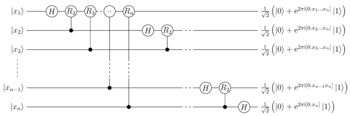
To obtain this state from the circuit depicted above, a swap operations of the qubits must be performed to reverse their order. At most ${\displaystyle n/2}$ swaps are required, each one being accomplished using three controlled-NOT (C-NOT) gates.^[2]

After the reversal, the n-th output qubit will be in a superposition state of ${\displaystyle |0\rangle }$ and ${\displaystyle e^{2\pi i\,[0.x_{1}...x_{n}]}|1\rangle }$, and similarly the other qubits before that (take a second look at the sketch of the circuit above).

In other words, the discrete Fourier transform, an operation on n qubits, can be factored into the tensor product of n single-qubit operations, suggesting it is easily represented as a quantum circuit (up to an order reversal of the output). In fact, each of those single-qubit operations can be implemented efficiently using a Hadamard gate and controlled phase gates. The first term requires one Hadamard gate and ${\displaystyle (n-1)}$ controlled phase gates, the next one requires a Hadamard gate and ${\displaystyle (n-2)}$ controlled phase gate, and each following term requires one fewer controlled phase gate. Summing up the number of gates, excluding the ones needed for the output reversal, gives ${\displaystyle n+(n-1)+\cdots +1=n(n+1)/2=O(n^{2})}$ gates, which is quadratic polynomial in the number of qubits.

Example[]

Consider the quantum Fourier transform on 3 qubits. It is the following transformation:

${\displaystyle {\text{QFT}}:|x\rangle \mapsto {\frac {1}{\sqrt {2^{3}}}}\sum _{k=0}^{2^{3}-1}\omega _{3}'^{xk}|k\rangle ,}$

where ${\displaystyle \omega _{3}'=\omega _{\left(2^{3}\right)}}$ is a primitive eighth root of unity satisfying ${\displaystyle \omega _{3}'^{8}=\left(e^{\frac {2\pi i}{2^{3}}}\right)^{8}=1}$ (since ${\displaystyle N=2^{3}=8}$).

For short, setting ${\displaystyle \omega =\omega _{3}'=\omega _{8}}$, the matrix representation of this transformation on 3 qubits is:

${\displaystyle F_{2^{3}}={\frac {1}{\sqrt {2^{3}}}}{\begin{bmatrix}1&1&1&1&1&1&1&1\\1&\omega &\omega ^{2}&\omega ^{3}&\omega ^{4}&\omega ^{5}&\omega ^{6}&\omega ^{7}\\1&\omega ^{2}&\omega ^{4}&\omega ^{6}&\omega ^{8}&\omega ^{10}&\omega ^{12}&\omega ^{14}\\1&\omega ^{3}&\omega ^{6}&\omega ^{9}&\omega ^{12}&\omega ^{15}&\omega ^{18}&\omega ^{21}\\1&\omega ^{4}&\omega ^{8}&\omega ^{12}&\omega ^{16}&\omega ^{20}&\omega ^{24}&\omega ^{28}\\1&\omega ^{5}&\omega ^{10}&\omega ^{15}&\omega ^{20}&\omega ^{25}&\omega ^{30}&\omega ^{35}\\1&\omega ^{6}&\omega ^{12}&\omega ^{18}&\omega ^{24}&\omega ^{30}&\omega ^{36}&\omega ^{42}\\1&\omega ^{7}&\omega ^{14}&\omega ^{21}&\omega ^{28}&\omega ^{35}&\omega ^{42}&\omega ^{49}\\\end{bmatrix}}={\frac {1}{\sqrt {2^{3}}}}{\begin{bmatrix}1&1&1&1&1&1&1&1\\1&\omega &\omega ^{2}&\omega ^{3}&\omega ^{4}&\omega ^{5}&\omega ^{6}&\omega ^{7}\\1&\omega ^{2}&\omega ^{4}&\omega ^{6}&1&\omega ^{2}&\omega ^{4}&\omega ^{6}\\1&\omega ^{3}&\omega ^{6}&\omega &\omega ^{4}&\omega ^{7}&\omega ^{2}&\omega ^{5}\\1&\omega ^{4}&1&\omega ^{4}&1&\omega ^{4}&1&\omega ^{4}\\1&\omega ^{5}&\omega ^{2}&\omega ^{7}&\omega ^{4}&\omega &\omega ^{6}&\omega ^{3}\\1&\omega ^{6}&\omega ^{4}&\omega ^{2}&1&\omega ^{6}&\omega ^{4}&\omega ^{2}\\1&\omega ^{7}&\omega ^{6}&\omega ^{5}&\omega ^{4}&\omega ^{3}&\omega ^{2}&\omega \\\end{bmatrix}}.}$

It could be simplified further by using ${\displaystyle \omega ^{4}=-1}$, ${\displaystyle \omega ^{2}=i}$ and ${\displaystyle \omega ^{6}=-i}$

and then even more given that ${\displaystyle \omega ^{5}=-\omega }$, ${\displaystyle \omega ^{3}=i\omega }$ and ${\displaystyle \omega ^{7}=-i\omega }$.

The 3-qubit quantum Fourier transform can be rewritten as:

${\displaystyle {\text{QFT}}(|x_{1},x_{2},x_{3}\rangle )={\frac {1}{\sqrt {2^{3}}}}\ \left(|0\rangle +e^{2\pi i\,[0.x_{3}]}|1\rangle \right)\otimes \left(|0\rangle +e^{2\pi i\,[0.x_{2}x_{3}]}|1\rangle \right)\otimes \left(|0\rangle +e^{2\pi i\,[0.x_{1}x_{2}x_{3}]}|1\rangle \right)}$

or

${\displaystyle {\text{QFT}}(|x_{1},x_{2},x_{3}\rangle )={\frac {1}{\sqrt {2^{3}}}}\ \left(|0\rangle +\omega _{1}'^{[x_{3}]}|1\rangle \right)\otimes \left(|0\rangle +\omega _{2}'^{[x_{2}x_{3}]}|1\rangle \right)\otimes \left(|0\rangle +\omega _{3}'^{[x_{1}x_{2}x_{3}]}|1\rangle \right).}$

In case that we use the circuit we obtain the factorization in reverse order, namely

${\displaystyle |x_{1},x_{2},x_{3}\rangle \longmapsto {\frac {1}{\sqrt {2^{3}}}}\ \left(|0\rangle +\omega _{3}'^{[x_{1}x_{2}x_{3}]}|1\rangle \right)\otimes \left(|0\rangle +\omega _{2}'^{[x_{2}x_{3}]}|1\rangle \right)\otimes \left(|0\rangle +\omega _{1}'^{[x_{3}]}|1\rangle \right).}$

Here we have used notations like:

${\displaystyle [0.x_{1}x_{2}x_{3}]=[x_{1}x_{2}x_{3}]/2^{3}}$and ${\displaystyle \omega _{m}'=\omega _{\left(2^{m}\right)}=e^{2\pi i/2^{m}}.}$

In the following sketch, we have the respective circuit for ${\displaystyle n=3}$ (with wrong order of output qubits with respect to the proper QFT):

As calculated above, the number of gates used is ${\displaystyle n(n+1)/2}$ which is equal to ${\displaystyle 6}$, for ${\displaystyle n=3}$.

Relation to quantum Hadamard transform[]

Using the generalized Fourier transform on finite (abelian) groups, there are actually two natural ways to define a quantum Fourier transform on an n-qubit quantum register. The QFT as defined above is equivalent to the DFT, which considers these n qubits as indexed by the cyclic group ${\displaystyle \mathbb {Z} /2^{n}\mathbb {Z} }$. However, it also makes sense to consider the qubits as indexed by the Boolean group ${\displaystyle (\mathbb {Z} /2\mathbb {Z} )^{n}}$, and in this case the Fourier transform is the Hadamard transform. This is achieved by applying a Hadamard gate to each of the n qubits in parallel.^[4][5] Note that Shor's algorithm uses both types of Fourier transforms, both an initial Hadamard transform as well as a QFT.

References[]

• K. R. Parthasarathy, Lectures on Quantum Computation and Quantum Error Correcting Codes (Indian Statistical Institute, Delhi Center, June 2001)
• John Preskill, Lecture Notes for Physics 229: Quantum Information and Computation (CIT, September 1998)

External links[]

• Wolfram Demonstration Project: Quantum Circuit Implementing Grover's Search Algorithm
• Wolfram Demonstration Project: Quantum Circuit Implementing Quantum Fourier Transform
• Quirk online life quantum fourier transform