Schrödinger equation

Part of a series of articles about
Quantum mechanics
${\displaystyle i\hbar {\frac {\partial }{\partial t}}|\psi (t)\rangle ={\hat {H}}|\psi (t)\rangle }$ Schrödinger equation
Introduction Glossary History
show Background Classical mechanics Old quantum theory Bra–ket notation Hamiltonian Interference
show Fundamentals Complementarity Decoherence Entanglement Energy level Measurement Nonlocality Quantum number State Superposition Symmetry Tunnelling Uncertainty Wave function (collapse)
show Experiments Bell's inequality Davisson–Germer Double-slit Elitzur–Vaidman Franck–Hertz Leggett–Garg inequality Mach–Zehnder Popper Quantum eraser (delayed-choice) Schrödinger's cat Stern–Gerlach Wheeler's delayed-choice
show Formulations Overview Heisenberg Interaction Matrix Phase-space Schrödinger Sum-over-histories (path integral)
hide Equations Dirac Klein–Gordon Pauli Rydberg Schrödinger
show Interpretations Overview Bayesian Consistent histories Copenhagen de Broglie–Bohm Ensemble Hidden-variable Many-worlds Objective collapse Quantum logic Relational Transactional
show Advanced topics Relativistic quantum mechanics Quantum field theory Quantum information science Quantum computing Quantum chaos Density matrix Scattering theory Quantum statistical mechanics Quantum machine learning
show Scientists Aharonov Bell Blackett Bloch Bohm Bohr Born Bose de Broglie Candlin Compton Dirac Davisson Debye Ehrenfest Einstein Everett Fock Fermi Feynman Glauber Gutzwiller Heisenberg Hilbert Jordan Kramers Pauli Lamb Landau Laue Moseley Millikan Onnes Planck Rabi Raman Rydberg Schrödinger Sommerfeld von Neumann Weyl Wien Wigner Zeeman Zeilinger
v t

Modern physics
${\displaystyle {\hat {H}}|\psi _{n}(t)\rangle =i\hbar {\frac {\partial }{\partial t}}|\psi _{n}(t)\rangle }$ ${\displaystyle {\frac {1}{{c}^{2}}}{\frac {{\partial }^{2}{\phi }_{n}}{{\partial t}^{2}}}-{{\nabla }^{2}{\phi }_{n}}+{\left({\frac {mc}{\hbar }}\right)}^{2}{\phi }_{n}=0}$ Manifold dynamics: Schrödinger and Klein–Gordon equations
show Founders Max Planck  · Albert Einstein  · Niels Bohr  · Max Born  · Werner Heisenberg  · Erwin Schrödinger  · Pascual Jordan  · Wolfgang Pauli  · Paul Dirac  · Ernest Rutherford  · Louis de Broglie  · Satyendra Nath Bose
show Concepts Topology · Space · Time · Energy · Matter · Work Randomness · Information · Entropy · Mind Light · Particle · Wave
show Branches Applied · Experimental · Theoretical Mathematical  · Philosophy of physics Quantum mechanics (Quantum field theory · Quantum information · Quantum computation) Electromagnetism · Weak interaction · Electroweak interaction Strong interaction Atomic · Particle · Nuclear Atomic, molecular, and optical Condensed matter · Statistical Complex systems · Non-linear dynamics · Biophysics Neurophysics Plasma physics Special relativity · General relativity Astrophysics · Cosmology Theories of gravitation Quantum gravity · Theory of everything
show Scientists Witten · Röntgen · Becquerel · Lorentz · Planck · Curie · Wien · Skłodowska-Curie · Sommerfeld · Rutherford · Soddy · Onnes · Einstein · Wilczek · Born · Weyl · Bohr · Kramers · Schrödinger · de Broglie · Laue · Bose · Compton · Pauli · Walton · Fermi · van der Waals · Heisenberg · Dyson · Zeeman · Moseley · Hilbert · Gödel · Jordan · Dirac · Wigner · Hawking · P. W. Anderson · Lemaître · Thomson · Poincaré · Wheeler · Penrose · Millikan · Nambu · von Neumann · Higgs · Hahn · Feynman · Yang · Lee · Lenard · Salam · 't Hooft · Veltman · Bell · Gell-Mann · J. J. Thomson  · Raman · Bragg · Bardeen · Shockley · Chadwick · Lawrence · Zeilinger · Goudsmit · Uhlenbeck
show Categories Modern physics
v t

Schrödinger's equation inscribed on the gravestone of Annemarie and Erwin Schrödinger. (Newton's dot notation for the time derivative is used.)

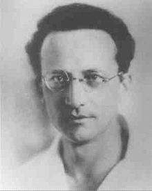
The Schrödinger equation is a linear partial differential equation that governs the wave function of a quantum-mechanical system.^[1]:1–2 It is a key result in quantum mechanics, and its discovery was a significant landmark in the development of the subject. The equation is named after Erwin Schrödinger, who postulated the equation in 1925, and published it in 1926, forming the basis for the work that resulted in his Nobel Prize in Physics in 1933.^[2][3]

Conceptually, the Schrödinger equation is the quantum counterpart of Newton's second law in classical mechanics. Given a set of known initial conditions, Newton's second law makes a mathematical prediction as to what path a given physical system will take over time. The Schrödinger equation gives the evolution over time of a wave function, the quantum-mechanical characterization of an isolated physical system. The equation can be derived from the fact that the time-evolution operator must be unitary, and must therefore be generated by the exponential of a self-adjoint operator, which is the quantum Hamiltonian.

The Schrödinger equation is not the only way to study quantum mechanical systems and make predictions. The other formulations of quantum mechanics include matrix mechanics, introduced by Werner Heisenberg, and the path integral formulation, developed chiefly by Richard Feynman. Paul Dirac incorporated matrix mechanics and the Schrödinger equation into a single formulation. When these approaches are compared, the use of the Schrödinger equation is sometimes called "wave mechanics".

Definition[]

Preliminaries[]

Complex plot of a wave function that satisfies the nonrelativistic Schrödinger equation with V = 0. In other words, this corresponds to a particle traveling freely through empty space.

Introductory courses on physics or chemistry typically introduce the Schrödinger equation in a way that can be appreciated knowing only the concepts and notations of basic calculus, particularly derivatives with respect to space and time. A special case of the Schrödinger equation that admits a statement in those terms is the position-space Schrödinger equation for a single nonrelativistic particle in one dimension:

${\displaystyle i\hbar {\frac {\partial }{\partial t}}\Psi (x,t)=\left[-{\frac {\hbar ^{2}}{2m}}{\frac {\partial ^{2}}{\partial x^{2}}}+V(x,t)\right]\Psi (x,t)\,.}$

Here, ${\displaystyle \Psi (x,t)}$ is a wave function, a function that assigns a complex number to each point ${\displaystyle x}$ at each time ${\displaystyle t}$. The parameter ${\displaystyle m}$ is the mass of the particle, and ${\displaystyle V(x,t)}$ is the potential that represents the environment in which the particle exists. The constant ${\displaystyle i}$ is the imaginary unit, and ${\displaystyle \hbar }$ is the reduced Planck constant, which has units of action (energy multiplied by time).

Broadening beyond this simple case, the mathematically rigorous formulation of quantum mechanics developed by Paul Dirac,^[4] David Hilbert,^[5] John von Neumann,^[6] and Hermann Weyl^[7] defines the state of a quantum mechanical system to be a vector ${\displaystyle |\psi \rangle }$ belonging to a (separable) Hilbert space ${\displaystyle {\mathcal {H}}}$. This vector is postulated to be normalized under the Hilbert's space inner product, that is, in Dirac notation it obeys ${\displaystyle \langle \psi |\psi \rangle =1}$. The exact nature of this Hilbert space is dependent on the system – for example, for describing position and momentum the Hilbert space is the space of complex square-integrable functions ${\displaystyle L^{2}(\mathbb {C} )}$, while the Hilbert space for the spin of a single proton is simply the space of two-dimensional complex vectors ${\displaystyle \mathbb {C} ^{2}}$ with the usual inner product.

Physical quantities of interest — position, momentum, energy, spin — are represented by "observables", which are Hermitian (more precisely, self-adjoint) linear operators acting on the Hilbert space. A wave function can be an eigenvector of an observable, in which case it is called an eigenstate, and the associated eigenvalue corresponds to the value of the observable in that eigenstate. More generally, a quantum state will be a linear combination of the eigenstates, known as a quantum superposition. When an observable is measured, the result will be one of its eigenvalues with probability given by the Born rule: in the simplest case the eigenvalue ${\displaystyle \lambda }$ is non-degenerate and the probability is given by ${\displaystyle |\langle \lambda |\psi \rangle |^{2}}$, where ${\displaystyle |\lambda \rangle }$ is its associated eigenvector. More generally, the eigenvalue is degenerate and the probability is given by ${\displaystyle \langle \psi |P_{\lambda }|\psi \rangle }$, where ${\displaystyle P_{\lambda }}$ is the projector onto its associated eigenspace.^{[note 1]}

A momentum eigenstate would be a perfectly monochromatic wave of infinite extent, which is not square-integrable. Likewise, a position eigenstate would be a Dirac delta distribution, not square-integrable and technically not a function at all. Consequently, neither can belong to the particle's Hilbert space. Physicists sometimes introduce fictitious "bases" for a Hilbert space comprising elements outside that space. These are invented for calculational convenience and do not represent physical states.^{[8]:100–105}

Time-dependent equation[]

The form of the Schrödinger equation depends on the physical situation. The most general form is the time-dependent Schrödinger equation, which gives a description of a system evolving with time:^[9]:143

where ${\displaystyle \Psi }$ (the Greek letter psi) is the state vector of the quantum system, ${\displaystyle t}$ is time, and ${\displaystyle {\hat {H}}}$ is an observable, the Hamiltonian operator.

Each of these three rows is a wave function which satisfies the time-dependent Schrödinger equation for a harmonic oscillator. Left: The real part (blue) and imaginary part (red) of the wave function. Right: The probability distribution of finding the particle with this wave function at a given position. The top two rows are examples of stationary states, which correspond to standing waves. The bottom row is an example of a state which is not a stationary state. The right column illustrates why stationary states are called "stationary".

The term "Schrödinger equation" can refer to both the general equation, or the specific nonrelativistic version. The general equation is indeed quite general, used throughout quantum mechanics, for everything from the Dirac equation to quantum field theory, by plugging in diverse expressions for the Hamiltonian. The specific nonrelativistic version is an approximation that yields accurate results in many situations, but only to a certain extent (see relativistic quantum mechanics and relativistic quantum field theory).

To apply the Schrödinger equation, write down the Hamiltonian for the system, accounting for the kinetic and potential energies of the particles constituting the system, then insert it into the Schrödinger equation. The resulting partial differential equation is solved for the wave function, which contains information about the system. In practice, the square of the absolute value of the wave function at each point is taken to define a probability density function. For example, given a wave function in position space ${\displaystyle \Psi (x,t)}$ as above, we have

${\displaystyle \mathrm {Pr} (x,t)=|\Psi (x,t)|^{2}.}$

Time-independent equation[]

The time-dependent Schrödinger equation described above predicts that wave functions can form standing waves, called stationary states. These states are particularly important as their individual study later simplifies the task of solving the time-dependent Schrödinger equation for any state. Stationary states can also be described by a simpler form of the Schrödinger equation, the time-independent Schrödinger equation.

where ${\displaystyle E}$ is the energy of the system. This is only used when the Hamiltonian itself is not dependent on time explicitly. However, even in this case the total wave function still has a time dependency. In the language of linear algebra, this equation is an eigenvalue equation. Therefore, the wave function is an eigenfunction of the Hamiltonian operator with corresponding eigenvalue(s) ${\displaystyle E}$.

Properties[]

Linearity[]

The Schrödinger equation is a linear differential equation, meaning that if two wave functions ψ₁ and ψ₂ are solutions, then so is any linear combination of the two:

${\displaystyle \displaystyle \psi =a\psi _{1}+b\psi _{2}}$

where a and b are any complex numbers.^[10]:25 Moreover, the sum can be extended for any number of wave functions. This property allows superpositions of quantum states to be solutions of the Schrödinger equation. Even more generally, it holds that a general solution to the Schrödinger equation can be found by taking a weighted sum over a basis of states. A choice often employed is the basis of energy eigenstates, which are solutions of the time-independent Schrödinger equation. For example, consider a wave function Ψ(x, t) such that the wave function is a product of two functions: one time independent, and one time dependent. If states of definite energy found using the time independent Schrödinger equation are given by ψ_E(x) with amplitude A_n and time dependent phase factor is given by

${\displaystyle e^{{-iE_{n}t}/\hbar },}$

then a valid general solution is

${\displaystyle \Psi (x,t)=\sum _{n}A_{n}\psi _{E_{n}}(x)e^{{-iE_{n}t}/\hbar }.}$

Unitarity[]

Holding the Hamiltonian ${\displaystyle {\hat {H}}}$ constant, the Schrödinger equation has the solution^[9]

${\displaystyle |\Psi (t)\rangle =e^{-i{\hat {H}}t/\hbar }|\Psi (0)\rangle \,.}$

The operator ${\displaystyle {\hat {U}}(t)=e^{-i{\hat {H}}t/\hbar }}$ is known as the time-evolution operator, and it is unitary: it preserves the inner product between vectors in the Hilbert space.^[10] Unitarity is a general feature of time evolution under the Schrödinger equation. If the initial state is ${\displaystyle |\Psi (0)\rangle }$, then the state at a later time ${\displaystyle t}$ will be given by

${\displaystyle |\Psi (t)\rangle ={\hat {U}}|\Psi (0)\rangle }$

for some unitary operator ${\displaystyle {\hat {U}}}$. Likewise, suppose that ${\displaystyle {\hat {U}}(t)}$ is a continuous family of unitary operators parameterized by ${\displaystyle t}$. Without loss of generality,^[11] the parameterization can be chosen so that ${\displaystyle {\hat {U}}(0)}$ is the identity operator and that ${\displaystyle {\hat {U}}(t/N)^{N}={\hat {U}}(t)}$ for any ${\displaystyle N>0}$. Then ${\displaystyle {\hat {U}}(t)}$ depends exponentially upon the parameter ${\displaystyle t}$, implying

${\displaystyle U(t)=e^{-i{\hat {G}}t}}$

for some self-adjoint operator ${\displaystyle {\hat {G}}}$, called the generator of the family ${\displaystyle {\hat {U}}(t)}$. A Hamiltonian is just such a generator (up to the factor of Planck's constant that would be set to 1 in natural units).

Changes of basis[]

The Schrödinger equation is often presented using quantities varying as functions of position, but as a vector-operator equation it has a valid representation in any arbitrary complete basis of kets in Hilbert space. As mentioned above, "bases" that lie outside the physical Hilbert space are also employed for calculational purposes. This is illustrated by the position-space and momentum-space Schrödinger equations for a nonrelativistic, spinless particle.^[8]:182 The Hilbert space for such a particle is the space of complex square-integrable functions on three-dimensional Euclidean space, and its Hamiltonian is the sum of a kinetic-energy term that is quadratic in the momentum operator and a potential-energy term:

${\displaystyle i\hbar {\frac {d}{dt}}|\Psi (t)\rangle =\left({\frac {1}{2m}}{\hat {p}}^{2}+{\hat {V}}\right)|\Psi (t)\rangle \,.}$

Writing ${\displaystyle \mathbf {r} }$ for a three-dimensional position vector and ${\displaystyle \mathbf {p} }$ for a three-dimensional momentum vector, the position-space Schrödinger equation is

${\displaystyle i\hbar {\frac {\partial }{\partial t}}\Psi (\mathbf {r} ,t)=-{\frac {\hbar ^{2}}{2m}}\nabla ^{2}\Psi (\mathbf {r} ,t)+V(\mathbf {r} )\Psi (\mathbf {r} ,t)\,.}$

The momentum-space counterpart involves the Fourier transforms of the wave function and the potential:

${\displaystyle i\hbar {\frac {\partial }{\partial t}}{\tilde {\Psi }}(\mathbf {p} ,t)={\frac {\mathbf {p} ^{2}}{2m}}{\tilde {\Psi }}(\mathbf {p} ,t)+(2\pi \hbar )^{-3/2}\int d^{3}\mathbf {p} '\,{\tilde {V}}(\mathbf {p} -\mathbf {p} '){\tilde {\Psi }}(\mathbf {p} ',t)\,.}$

The functions ${\displaystyle \Psi (\mathbf {r} ,t)}$ and ${\displaystyle {\tilde {\Psi }}(\mathbf {p} ,t)}$ are derived from ${\displaystyle |\Psi (t)\rangle }$ by

${\displaystyle \Psi (\mathbf {r} ,t)=\langle \mathbf {r} |\Psi (t)\rangle \,,}$

${\displaystyle {\tilde {\Psi }}(\mathbf {p} ,t)=\langle \mathbf {p} |\Psi (t)\rangle \,,}$

where ${\displaystyle |\mathbf {r} \rangle }$ and ${\displaystyle |\mathbf {p} \rangle }$ do not belong to the Hilbert space itself, but have well-defined inner products with all elements of that space.

When restricted from three dimensions to one, the position-space equation is just the first form of the Schrödinger equation given above. The relation between position and momentum in quantum mechanics can be appreciated in a single dimension. In canonical quantization, the classical variables ${\displaystyle x}$ and ${\displaystyle p}$ are promoted to self-adjoint operators ${\displaystyle {\hat {x}}}$ and ${\displaystyle {\hat {p}}}$ that satisfy the canonical commutation relation

${\displaystyle [{\hat {x}},{\hat {p}}]=i\hbar \,.}$

This implies that^[8]:190

${\displaystyle \langle x|{\hat {p}}|\Psi \rangle =-i\hbar {\frac {d}{dx}}\Psi (x)\,,}$

so the action of the momentum operator ${\displaystyle {\hat {p}}}$ in the position-space representation is ${\displaystyle -i\hbar {\frac {d}{dx}}}$. Thus, ${\displaystyle {\hat {p}}^{2}}$ becomes a second derivative, and in three dimensions, the second derivative becomes the Laplacian ${\displaystyle \nabla ^{2}}$.

The canonical commutation relation also implies that the position and momentum operators are Fourier conjugates of each other. Consequently, functions originally defined in terms of their position dependence can be converted to functions of momentum using the Fourier transform. In solid-state physics, the Schrödinger equation is often written for functions of momentum, as Bloch's theorem ensures the periodic crystal lattice potential couples ${\displaystyle {\tilde {\Psi }}(p)}$ with ${\displaystyle {\tilde {\Psi }}(p+K)}$ for only discrete reciprocal lattice vectors ${\displaystyle K}$. This makes it convenient to solve the momentum-space Schrödinger equation at each point in the Brillouin zone independently of the other points in the Brillouin zone.

Probability current[]

The Schrödinger equation is consistent with local probability conservation.^[8]:238 Multiplying the Schrödinger equation on the right by the complex conjugate wave function, and multiplying the wave function to the left of the complex conjugate of the Schrödinger equation, and subtracting, gives the continuity equation for probability:

${\displaystyle {\partial \over \partial t}\rho \left(\mathbf {r} ,t\right)+\nabla \cdot \mathbf {j} =0,}$

where

${\displaystyle \rho =|\Psi |^{2}=\Psi ^{*}(\mathbf {r} ,t)\Psi (\mathbf {r} ,t)\,\!}$

is the probability density (probability per unit volume, * denotes complex conjugate), and

${\displaystyle \mathbf {j} ={1 \over 2m}\left(\Psi ^{*}{\hat {\mathbf {p} }}\Psi -\Psi {\hat {\mathbf {p} }}\Psi ^{*}\right)\,\!}$

is the probability current (flow per unit area).

Separation of variables[]

If the Hamiltonian is not an explicit function of time, the equation is separable into a product of spatial and temporal parts. In general, the wave function takes the form:

${\displaystyle \Psi (\mathbf {r} ,t)=\psi (\mathbf {r} )\tau (t)\,.}$

where ${\displaystyle \psi (\mathbf {r} )}$ is a function of all the spatial coordinate(s) of the particle(s) constituting the system only, and ${\displaystyle \tau (t)}$ is a function of time only. Substituting this expression for ${\displaystyle \Psi }$ into the Schrödinger equation and solving by separation of variables implies the general solution of the time-dependent equation has the form

${\displaystyle \Psi (\mathbf {r} ,t)=\psi (\mathbf {r} )e^{-i{Et/\hbar }}\,.}$

Since the time dependent phase factor is always the same, only the spatial part needs to be solved for in time-independent problems. Additionally, the energy operator Ĥ = iħ∂/∂t can always be replaced by the energy eigenvalue E, and thus the time-independent Schrödinger equation is an eigenvalue equation for the Hamiltonian operator:^[9]:143ff

${\displaystyle {\hat {H}}\psi =E\psi }$

This is true for any number of particles in any number of dimensions (in a time-independent potential). This case describes the standing wave solutions of the time-dependent equation, which are the states with definite energy (instead of a probability distribution of different energies). In physics, these standing waves are called "stationary states" or "energy eigenstates"; in chemistry they are called "atomic orbitals" or "molecular orbitals". Superpositions of energy eigenstates change their properties according to the relative phases between the energy levels. The energy eigenstates form a basis: any wave function may be written as a sum over the discrete energy states or an integral over continuous energy states, or more generally as an integral over a measure. This is the spectral theorem in mathematics, and in a finite state space it is just a statement of the completeness of the eigenvectors of a Hermitian matrix.

Separation of variables can also be a useful method for the time-independent Schrödinger equation. For example, depending on the symmetry of the problem, the Cartesian axes might be separated,

${\displaystyle \psi (\mathbf {r} )=\psi _{x}(x)\psi _{y}(y)\psi _{z}(z)\,,}$

or radial and angular coordinates might be separated:

${\displaystyle \psi (\mathbf {r} )=\psi _{r}(r)\psi _{\theta }(\theta )\psi _{\phi }(\phi )\,.}$

Examples[]

Particle in a box[]

1-dimensional potential energy box (or infinite potential well)

The particle in a one-dimensional potential energy box is the most mathematically simple example where restraints lead to the quantization of energy levels. The box is defined as having zero potential energy inside a certain region and infinite potential energy outside.^[8]:77–78 For the one-dimensional case in the ${\displaystyle x}$ direction, the time-independent Schrödinger equation may be written

${\displaystyle -{\frac {\hbar ^{2}}{2m}}{\frac {d^{2}\psi }{dx^{2}}}=E\psi .}$

With the differential operator defined by

${\displaystyle {\hat {p}}_{x}=-i\hbar {\frac {d}{dx}}}$

the previous equation is evocative of the classic kinetic energy analogue,

${\displaystyle {\frac {1}{2m}}{\hat {p}}_{x}^{2}=E,}$

with state ${\displaystyle \psi }$ in this case having energy ${\displaystyle E}$ coincident with the kinetic energy of the particle.

The general solutions of the Schrödinger equation for the particle in a box are

${\displaystyle \psi (x)=Ae^{ikx}+Be^{-ikx}\qquad \qquad E={\frac {\hbar ^{2}k^{2}}{2m}}}$

or, from Euler's formula,

${\displaystyle \psi (x)=C\sin(kx)+D\cos(kx).\!}$

The infinite potential walls of the box determine the values of ${\displaystyle C,D,}$ and ${\displaystyle k}$ at ${\displaystyle x=0}$ and ${\displaystyle x=L}$ where ${\displaystyle \psi }$ must be zero. Thus, at ${\displaystyle x=0}$,

${\displaystyle \psi (0)=0=C\sin(0)+D\cos(0)=D}$

and ${\displaystyle D=0}$. At ${\displaystyle x=L}$,

${\displaystyle \psi (L)=0=C\sin(kL),}$

in which ${\displaystyle C}$ cannot be zero as this would conflict with the postulate that ${\displaystyle \psi }$ has norm 1. Therefore, since ${\displaystyle \sin(kL)=0}$, ${\displaystyle kL}$ must be an integer multiple of ${\displaystyle \pi }$,

${\displaystyle k={\frac {n\pi }{L}}\qquad \qquad n=1,2,3,\ldots .}$

This constraint on ${\displaystyle k}$ implies a constraint on the energy levels, yielding

${\displaystyle E_{n}={\frac {\hbar ^{2}\pi ^{2}n^{2}}{2mL^{2}}}={\frac {n^{2}h^{2}}{8mL^{2}}}.}$

A finite potential well is the generalization of the infinite potential well problem to potential wells having finite depth. The finite potential well problem is mathematically more complicated than the infinite particle-in-a-box problem as the wave function is not pinned to zero at the walls of the well. Instead, the wave function must satisfy more complicated mathematical boundary conditions as it is nonzero in regions outside the well. Another related problem is that of the rectangular potential barrier, which furnishes a model for the quantum tunneling effect that plays an important role in the performance of modern technologies such as flash memory and scanning tunneling microscopy.

Harmonic oscillator[]

A harmonic oscillator in classical mechanics (A–B) and quantum mechanics (C–H). In (A–B), a ball, attached to a spring, oscillates back and forth. (C–H) are six solutions to the Schrödinger Equation for this situation. The horizontal axis is position, the vertical axis is the real part (blue) or imaginary part (red) of the wave function. Stationary states, or energy eigenstates, which are solutions to the time-independent Schrödinger equation, are shown in C, D, E, F, but not G or H.

The Schrödinger equation for this situation is

${\displaystyle E\psi =-{\frac {\hbar ^{2}}{2m}}{\frac {d^{2}}{dx^{2}}}\psi +{\frac {1}{2}}m\omega ^{2}x^{2}\psi ,}$

where ${\displaystyle x}$ is the displacement and ${\displaystyle \omega }$ the angular frequency. This is an example of a quantum-mechanical system whose wave function can be solved for exactly. Furthermore, it can be used to describe approximately a wide variety of other systems, including vibrating atoms, molecules,^[12] and atoms or ions in lattices,^[13] and approximating other potentials near equilibrium points. It is also the basis of perturbation methods in quantum mechanics.

The solutions in position space are

${\displaystyle \psi _{n}(x)={\sqrt {\frac {1}{2^{n}\,n!}}}\cdot \left({\frac {m\omega }{\pi \hbar }}\right)^{1/4}\cdot e^{-{\frac {m\omega x^{2}}{2\hbar }}}\cdot {\mathcal {H}}_{n}\left({\sqrt {\frac {m\omega }{\hbar }}}x\right),}$

where ${\displaystyle n\in \{0,1,2,\ldots \}}$, and the functions ${\displaystyle {\mathcal {H}}_{n}}$ are the Hermite polynomials of order ${\displaystyle n}$. The solution set may be generated by

${\displaystyle \psi _{n}(x)={\frac {1}{\sqrt {n!}}}\left({\sqrt {\frac {m\omega }{2\hbar }}}\right)^{n}\left(x-{\frac {\hbar }{m\omega }}{\frac {d}{dx}}\right)^{n}\left({\frac {m\omega }{\pi \hbar }}\right)^{\frac {1}{4}}e^{\frac {-m\omega x^{2}}{2\hbar }}.}$

The eigenvalues are

${\displaystyle E_{n}=\left(n+{\frac {1}{2}}\right)\hbar \omega .}$

The case ${\displaystyle n=0}$ is called the ground state, its energy is called the zero-point energy, and the wave function is a Gaussian.^[14]

The harmonic oscillator, like the particle in a box, illustrates the generic feature of the Schrödinger equation that the energies of bound eigenstates are discretized.^[8]:352

Hydrogen atom[]

The Schrödinger equation for the hydrogen atom (or a hydrogen-like atom) is

${\displaystyle E\psi =-{\frac {\hbar ^{2}}{2\mu }}\nabla ^{2}\psi -{\frac {q^{2}}{4\pi \varepsilon _{0}r}}\psi }$

where ${\displaystyle q}$ is the electron charge, ${\displaystyle \mathbf {r} }$ is the position of the electron relative to the nucleus, ${\displaystyle r=|\mathbf {r} |}$ is the magnitude of the relative position, the potential term is due to the Coulomb interaction, wherein ${\displaystyle \varepsilon _{0}}$ is the permittivity of free space and

${\displaystyle \mu ={\frac {m_{q}m_{p}}{m_{q}+m_{p}}}}$

is the 2-body reduced mass of the hydrogen nucleus (just a proton) of mass ${\displaystyle m_{p}}$ and the electron of mass ${\displaystyle m_{q}}$. The negative sign arises in the potential term since the proton and electron are oppositely charged. The reduced mass in place of the electron mass is used since the electron and proton together orbit each other about a common centre of mass, and constitute a two-body problem to solve. The motion of the electron is of principle interest here, so the equivalent one-body problem is the motion of the electron using the reduced mass.

The Schrödinger equation for a hydrogen atom can be solved by separation of variables.^[15] In this case, spherical polar coordinates are the most convenient. Thus,

${\displaystyle \psi (r,\theta ,\varphi )=R(r)Y_{\ell }^{m}(\theta ,\varphi )=R(r)\Theta (\theta )\Phi (\varphi ),}$

where R are radial functions and ${\displaystyle Y_{l}^{m}(\theta ,\varphi )}$ are spherical harmonics of degree ${\displaystyle \ell }$ and order ${\displaystyle m}$. This is the only atom for which the Schrödinger equation has been solved for exactly. Multi-electron atoms require approximate methods. The family of solutions are:^[16]

${\displaystyle \psi _{n\ell m}(r,\theta ,\varphi )={\sqrt {\left({\frac {2}{na_{0}}}\right)^{3}{\frac {(n-\ell -1)!}{2n[(n+\ell )!]}}}}e^{-r/na_{0}}\left({\frac {2r}{na_{0}}}\right)^{\ell }L_{n-\ell -1}^{2\ell +1}\left({\frac {2r}{na_{0}}}\right)\cdot Y_{\ell }^{m}(\theta ,\varphi )}$

where:

• ${\displaystyle a_{0}={\frac {4\pi \varepsilon _{0}\hbar ^{2}}{m_{q}q^{2}}}}$ is the Bohr radius,
• ${\displaystyle L_{n-\ell -1}^{2\ell +1}(\cdots )}$ are the generalized Laguerre polynomials of degree ${\displaystyle n-\ell -1}$.
• ${\displaystyle n,\ell ,m}$ are the principal, azimuthal, and magnetic quantum numbers respectively, which take the values:

${\displaystyle {\begin{aligned}n&=1,2,3,\dots \\\ell &=0,1,2,\dots ,n-1\\m&=-\ell ,\dots ,\ell \\\end{aligned}}}$

Approximate solutions[]

It is typically not possible to solve the Schrödinger equation exactly for situations of physical interest. Accordingly, approximate solutions are obtained using techniques like variational methods and WKB approximation. It is also common to treat a problem of interest as a small modification to a problem that can be solved exactly, a method known as perturbation theory.

Semiclassical limit[]

One simple way to compare classical to quantum mechanics is to consider the time-evolution of the expected position and expected momentum, which can then be compared to the time-evolution of the ordinary position and momentum in classical mechanics.^[17]:302 The quantum expectation values satisfy the Ehrenfest theorem. For a one-dimensional quantum particle moving in a potential ${\displaystyle V}$, the Ehrenfest theorem says

${\displaystyle m{\frac {d}{dt}}\langle x\rangle =\langle p\rangle ;\quad {\frac {d}{dt}}\langle p\rangle =-\left\langle V'(X)\right\rangle \,.}$

Although the first of these equations is consistent with the classical behavior, the second is not: If the pair ${\displaystyle (\langle X\rangle ,\langle P\rangle )}$ were to satisfy Newton's second law, the right-hand side of the second equation would have to be

${\displaystyle -V'\left(\left\langle X\right\rangle \right)\,}$

which is typically not the same as ${\displaystyle -\left\langle V'(X)\right\rangle }$. In the case of the quantum harmonic oscillator, however, ${\displaystyle V'}$ is linear and this distinction disappears, so that in this very special case, the expected position and expected momentum do exactly follow the classical trajectories.

For general systems, the best we can hope for is that the expected position and momentum will approximately follow the classical trajectories. If the wave function is highly concentrated around a point ${\displaystyle x_{0}}$, then ${\displaystyle V'\left(\left\langle X\right\rangle \right)}$ and ${\displaystyle \left\langle V'(X)\right\rangle }$ will be almost the same, since both will be approximately equal to ${\displaystyle V'(x_{0})}$. In that case, the expected position and expected momentum will remain very close to the classical trajectories, at least for as long as the wave function remains highly localized in position.

The Schrödinger equation in its general form

${\displaystyle i\hbar {\frac {\partial }{\partial t}}\Psi \left(\mathbf {r} ,t\right)={\hat {H}}\Psi \left(\mathbf {r} ,t\right)}$

is closely related to the Hamilton–Jacobi equation (HJE)

${\displaystyle -{\frac {\partial }{\partial t}}S(q_{i},t)=H\left(q_{i},{\frac {\partial S}{\partial q_{i}}},t\right)}$

where ${\displaystyle S}$ is the classical action and ${\displaystyle H}$ is the Hamiltonian function (not operator).^[17]:308 Here the generalized coordinates ${\displaystyle q_{i}}$ for ${\displaystyle i=1,2,3}$ (used in the context of the HJE) can be set to the position in Cartesian coordinates as ${\displaystyle \mathbf {r} =(q_{1},q_{2},q_{3})=(x,y,z)}$.

Substituting

${\displaystyle \Psi ={\sqrt {\rho (\mathbf {r} ,t)}}e^{iS(\mathbf {r} ,t)/\hbar }}$

where ${\displaystyle \rho }$ is the probability density, into the Schrödinger equation and then taking the limit ${\displaystyle \hbar \longrightarrow 0}$ in the resulting equation yield the Hamilton–Jacobi equation.

Density matrices[]

Wave functions are not always the most convenient way to describe quantum systems and their behavior. When the preparation of a system is only imperfectly known, or when the system under investigation is a part of a larger whole, density matrices may be used instead.^[17]:74 A density matrix is a positive semi-definite operator whose trace is equal to 1. (The term "density operator" is also used, particularly when the underlying Hilbert space is infinite-dimensional.) The set of all density matrices is convex, and the extreme points are the operators that project onto vectors in the Hilbert space. These are the density-matrix representations of wave functions; in Dirac notation, they are written

${\displaystyle {\hat {\rho }}=|\Psi \rangle \langle \Psi |\,.}$

The density-matrix analogue of the Schrödinger equation for wave functions is^[18][19]

${\displaystyle i\hbar {\frac {\partial {\hat {\rho }}}{\partial t}}=[{\hat {H}},{\hat {\rho }}]\,,}$

where the brackets denote a commutator. This is variously known as the von Neumann equation, the Liouville–von Neumann equation, or just the Schrödinger equation for density matrices.^[17]:312 If the Hamiltonian is time-independent, this equation can be easily solved to yield

${\displaystyle {\hat {\rho }}(t)=e^{-i{\hat {H}}t/\hbar }{\hat {\rho }}(0)e^{i{\hat {H}}t/\hbar }\,.}$

More generally, if the unitary operator ${\displaystyle {\hat {U}}(t)}$ describes wave function evolution over some time interval, then the time evolution of a density matrix over that same interval is given by

${\displaystyle {\hat {\rho }}(t)={\hat {U}}(t){\hat {\rho }}(0){\hat {U}}(t)^{\dagger }\,.}$

Unitary evolution of a density matrix conserves its von Neumann entropy.^[17]:267

Relativistic quantum physics and quantum field theory[]

Quantum field theory (QFT) is a framework that allows the combination of quantum mechanics with special relativity. The general form of the Schrödinger equation is also valid in QFT, both in relativistic and nonrelativistic situations.

Klein–Gordon and Dirac equations[]

Relativistic quantum mechanics is obtained where quantum mechanics and special relativity simultaneously apply. In general, one wishes to build relativistic wave equations from the relativistic energy–momentum relation

${\displaystyle E^{2}=(pc)^{2}+(m_{0}c^{2})^{2}\,,}$

instead of classical energy equations. The Klein–Gordon equation and the Dirac equation are two such equations. The Klein–Gordon equation,

${\displaystyle {\frac {1}{c^{2}}}{\frac {\partial ^{2}}{\partial t^{2}}}\psi -\nabla ^{2}\psi +{\frac {m^{2}c^{2}}{\hbar ^{2}}}\psi =0.}$,

was the first such equation to be obtained, even before the nonrelativistic one, and applies to massive spinless particles. The Dirac equation arose from taking the "square root" of the Klein–Gordon equation by factorizing the entire relativistic wave operator into a product of two operators – one of these is the operator for the entire Dirac equation. Entire Dirac equation:

${\displaystyle \left(\beta mc^{2}+c\left(\sum _{n\mathop {=} 1}^{3}\alpha _{n}p_{n}\right)\right)\psi =i\hbar {\frac {\partial \psi }{\partial t}}}$

The general form of the Schrödinger equation remains true in relativity, but the Hamiltonian is less obvious. For example, the Dirac Hamiltonian for a particle of mass m and electric charge q in an electromagnetic field (described by the electromagnetic potentials φ and A) is:

${\displaystyle {\hat {H}}_{\text{Dirac}}=\gamma ^{0}\left[c{\boldsymbol {\gamma }}\cdot \left({\hat {\mathbf {p} }}-q\mathbf {A} \right)+mc^{2}+\gamma ^{0}q\varphi \right]\,,}$

in which the γ = (γ¹, γ², γ³) and γ⁰ are the Dirac gamma matrices related to the spin of the particle. The Dirac equation is true for all spin-1⁄2 particles, and the solutions to the equation are 4-component spinor fields with two components corresponding to the particle and the other two for the antiparticle.

For the Klein–Gordon equation, the general form of the Schrödinger equation is inconvenient to use, and in practice the Hamiltonian is not expressed in an analogous way to the Dirac Hamiltonian. The equations for relativistic quantum fields can be obtained in other ways, such as starting from a Lagrangian density and using the Euler–Lagrange equations for fields, or use the representation theory of the Lorentz group in which certain representations can be used to fix the equation for a free particle of given spin (and mass).

In general, the Hamiltonian to be substituted in the general Schrödinger equation is not just a function of the position and momentum operators (and possibly time), but also of spin matrices. Also, the solutions to a relativistic wave equation, for a massive particle of spin s, are complex-valued 2(2s + 1)-component spinor fields.

Fock space[]

As originally formulated, the Dirac equation is an equation for a single quantum particle, just like the single-particle Schrödinger equation with wave function ${\displaystyle \Psi (x,t)}$. This is of limited use in relativistic quantum mechanics, where particle number is not fixed. Heuristically, this complication can be motivated by noting that mass–energy equivalence implies material particles can be created from energy. A common way to address this in QFT is to introduce a Hilbert space where the basis states are labeled by particle number, a so-called Fock space. The Schrödinger equation can then be formulated for quantum states on this Hilbert space.^[20]

History[]

Erwin Schrödinger

Following Max Planck's quantization of light (see black-body radiation), Albert Einstein interpreted Planck's quanta to be photons, particles of light, and proposed that the energy of a photon is proportional to its frequency, one of the first signs of wave–particle duality. Since energy and momentum are related in the same way as frequency and wave number in special relativity, it followed that the momentum ${\displaystyle p}$ of a photon is inversely proportional to its wavelength ${\displaystyle \lambda }$, or proportional to its wave number ${\displaystyle k}$:

${\displaystyle p={\frac {h}{\lambda }}=\hbar k,}$

where ${\displaystyle h}$ is Planck's constant and ${\displaystyle \hbar ={h}/{2\pi }}$ is the reduced Planck constant. Louis de Broglie hypothesized that this is true for all particles, even particles which have mass such as electrons. He showed that, assuming that the matter waves propagate along with their particle counterparts, electrons form standing waves, meaning that only certain discrete rotational frequencies about the nucleus of an atom are allowed.^[21] These quantized orbits correspond to discrete energy levels, and de Broglie reproduced the Bohr model formula for the energy levels. The Bohr model was based on the assumed quantization of angular momentum ${\displaystyle L}$ according to:

${\displaystyle L=n{h \over 2\pi }=n\hbar .}$

According to de Broglie the electron is described by a wave and a whole number of wavelengths must fit along the circumference of the electron's orbit:

${\displaystyle n\lambda =2\pi r.\,}$

This approach essentially confined the electron wave in one dimension, along a circular orbit of radius ${\displaystyle r}$.

In 1921, prior to de Broglie, Arthur C. Lunn at the University of Chicago had used the same argument based on the completion of the relativistic energy–momentum 4-vector to derive what we now call the de Broglie relation.^[22][23] Unlike de Broglie, Lunn went on to formulate the differential equation now known as the Schrödinger equation, and solve for its energy eigenvalues for the hydrogen atom. Unfortunately the paper was rejected by the Physical Review, as recounted by Kamen.^[24]

Following up on de Broglie's ideas, physicist Peter Debye made an offhand comment that if particles behaved as waves, they should satisfy some sort of wave equation. Inspired by Debye's remark, Schrödinger decided to find a proper 3-dimensional wave equation for the electron. He was guided by William Rowan Hamilton's analogy between mechanics and optics, encoded in the observation that the zero-wavelength limit of optics resembles a mechanical system—the trajectories of light rays become sharp tracks that obey Fermat's principle, an analog of the principle of least action.^[25]

The equation he found is:^[26]

${\displaystyle i\hbar {\frac {\partial }{\partial t}}\Psi (\mathbf {r} ,\,t)=-{\frac {\hbar ^{2}}{2m}}\nabla ^{2}\Psi (\mathbf {r} ,\,t)+V(\mathbf {r} )\Psi (\mathbf {r} ,\,t).}$

However, by that time, Arnold Sommerfeld had refined the Bohr model with relativistic corrections.^[27][28] Schrödinger used the relativistic energy–momentum relation to find what is now known as the Klein–Gordon equation in a Coulomb potential (in natural units):

${\displaystyle \left(E+{e^{2} \over r}\right)^{2}\psi (x)=-\nabla ^{2}\psi (x)+m^{2}\psi (x).}$

He found the standing waves of this relativistic equation, but the relativistic corrections disagreed with Sommerfeld's formula. Discouraged, he put away his calculations and secluded himself with a mistress in a mountain cabin in December 1925.^[29]

While at the cabin, Schrödinger decided that his earlier nonrelativistic calculations were novel enough to publish, and decided to leave off the problem of relativistic corrections for the future. Despite the difficulties in solving the differential equation for hydrogen (he had sought help from his friend the mathematician Hermann Weyl^[30]:3) Schrödinger showed that his nonrelativistic version of the wave equation produced the correct spectral energies of hydrogen in a paper published in 1926.^[30]:1[31] Schrödinger computed the hydrogen spectral series by treating a hydrogen atom's electron as a wave ${\displaystyle \Psi (\mathbf {x} ,t)}$, moving in a potential well ${\displaystyle V}$, created by the proton. This computation accurately reproduced the energy levels of the Bohr model. In a paper, Schrödinger himself explained this equation as follows:

The already ... mentioned psi-function.... is now the means for predicting probability of measurement results. In it is embodied the momentarily attained sum of theoretically based future expectation, somewhat as laid down in a catalog.

— Erwin Schrödinger^[32]

The Schrödinger equation details the behavior of ${\displaystyle \Psi }$ but says nothing of its nature. Schrödinger tried to interpret its modulus squared as a charge density in a fourth paper, but he was unsuccessful.^[33]:219 In 1926, just a few days after this paper was published, Max Born successfully interpreted ${\displaystyle \Psi }$ as the probability amplitude, whose modulus squared is equal to probability density.^[33]:220

Interpretation[]

The Schrödinger equation provides a way to calculate the wave function of a system and how it changes dynamically in time. However, the Schrödinger equation does not directly say what, exactly, the wave function is. The meaning of the Schrödinger equation and how the mathematical entities in it relate to physical reality depends upon the interpretation of quantum mechanics that one adopts.

In the views often grouped together as the Copenhagen interpretation, a system's wave function is a collection of statistical information about that system. The Schrödinger equation relates information about the system at one time to information about it at another. While the time-evolution process represented by the Schrödinger equation is continuous and deterministic, in that knowing the wave function at one instant is in principle sufficient to calculate it for all future times, wave functions can also change discontinuously and stochastically during a measurement. The wave function changes, according to this school of thought, because new information is available. The post-measurement wave function generally cannot be known prior to the measurement, but the probabilities for the different possibilities can be calculated using the Born rule.^{[17][34][note 2]} Other, more recent interpretations of quantum mechanics, such as relational quantum mechanics and QBism also give the Schrödinger equation a status of this sort.^[37][38]

Schrödinger himself suggested in 1952 that the different terms of a superposition evolving under the Schrödinger equation are "not alternatives but all really happen simultaneously". This has been interpreted as an early version of Everett's many-worlds interpretation.^[39][40] This interpretation, formulated independently in 1956, holds that all the possibilities described by quantum theory simultaneously occur in a multiverse composed of mostly independent parallel universes.^[41] This interpretation removes the axiom of wave function collapse, leaving only continuous evolution under the Schrödinger equation, and so all possible states of the measured system and the measuring apparatus, together with the observer, are present in a real physical quantum superposition. While the multiverse is deterministic, we perceive non-deterministic behavior governed by probabilities, because we don't observe the multiverse as a whole, but only one parallel universe at a time. Exactly how this is supposed to work has been the subject of much debate. Why we should assign probabilities at all to outcomes that are certain to occur in some worlds, and why should the probabilities be given by the Born rule?^[42] Several ways to answer these questions in the many-worlds framework have been proposed, but there is no consensus on whether they are successful.^[43][44][45]

Bohmian mechanics reformulates quantum mechanics to make it deterministic, at the price of making it explicitly nonlocal (a price exacted by Bell's theorem). It attributes to each physical system not only a wave function but in addition a real position that evolves deterministically under a nonlocal guiding equation. The evolution of a physical system is given at all times by the Schrödinger equation together with the guiding equation.^[46]

See also[]

Notes[]

References[]

External links[]

Wikiquote has quotations related to: Schrödinger equation

• "Schrödinger equation". Encyclopedia of Mathematics. EMS Press. 2001 [1994].
• Quantum Cook Book and PHYS 201: Fundamentals of Physics II by Ramamurti Shankar, Yale OpenCourseware
• The Modern Revolution in Physics – an online textbook.
• Quantum Physics I at MIT OpenCourseWare