Vector field representation in 3D curvilinear coordinate systems
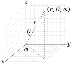
Spherical coordinates (
r,
θ,
φ) as commonly used in
physics: radial distance
r, polar angle
θ (
theta), and azimuthal angle
φ (
phi). The symbol
ρ (
rho) is often used instead of
r.
Note: This page uses common physics notation for spherical coordinates, in which
is the angle between the z axis and the radius vector connecting the origin to the point in question, while
is the angle between the projection of the radius vector onto the x-y plane and the x axis. Several other definitions are in use, and so care must be taken in comparing different sources.[1]
Cylindrical coordinate system[]
Vector fields[]
Vectors are defined in cylindrical coordinates by (ρ, φ, z), where
- ρ is the length of the vector projected onto the xy-plane,
- φ is the angle between the projection of the vector onto the xy-plane (i.e. ρ) and the positive x-axis (0 ≤ φ < 2π),
- z is the regular z-coordinate.
(ρ, φ, z) is given in Cartesian coordinates by:
![{\displaystyle {\begin{bmatrix}\rho \\\phi \\z\end{bmatrix}}={\begin{bmatrix}{\sqrt {x^{2}+y^{2}}}\\\operatorname {arctan} (y/x)\\z\end{bmatrix}},\ \ \ 0\leq \phi <2\pi ,}](https://wikimedia.org/api/rest_v1/media/math/render/svg/aceb22db9f623a755f979a239b6253f7ee5f4bb6)
or inversely by:
![{\displaystyle {\begin{bmatrix}x\\y\\z\end{bmatrix}}={\begin{bmatrix}\rho \cos \phi \\\rho \sin \phi \\z\end{bmatrix}}.}](https://wikimedia.org/api/rest_v1/media/math/render/svg/cff0ba0d806bb83b55a0c28df3bf558385dd6f1e)
Any vector field can be written in terms of the unit vectors as:
![{\displaystyle \mathbf {A} =A_{x}\mathbf {\hat {x}} +A_{y}\mathbf {\hat {y}} +A_{z}\mathbf {\hat {z}} =A_{\rho }\mathbf {\hat {\rho }} +A_{\phi }{\boldsymbol {\hat {\phi }}}+A_{z}\mathbf {\hat {z}} }](https://wikimedia.org/api/rest_v1/media/math/render/svg/9134a990d20a823aa85f14339c26d3e0ee6752b5)
The cylindrical unit vectors are related to the Cartesian unit vectors by:
![{\displaystyle {\begin{bmatrix}\mathbf {\hat {\rho }} \\{\boldsymbol {\hat {\phi }}}\\\mathbf {\hat {z}} \end{bmatrix}}={\begin{bmatrix}\cos \phi &\sin \phi &0\\-\sin \phi &\cos \phi &0\\0&0&1\end{bmatrix}}{\begin{bmatrix}\mathbf {\hat {x}} \\\mathbf {\hat {y}} \\\mathbf {\hat {z}} \end{bmatrix}}}](https://wikimedia.org/api/rest_v1/media/math/render/svg/0f83fe8b74d3cdf51e9ce9e12880e7beb5faa75b)
Note: the matrix is an orthogonal matrix, that is, its inverse is simply its transpose.
Time derivative of a vector field[]
To find out how the vector field A changes in time, the time derivatives should be calculated.
For this purpose Newton's notation will be used for the time derivative (
).
In Cartesian coordinates this is simply:
![{\dot {{\mathbf {A}}}}={\dot {A}}_{x}{\hat {{\mathbf {x}}}}+{\dot {A}}_{y}{\hat {{\mathbf {y}}}}+{\dot {A}}_{z}{\hat {{\mathbf {z}}}}](https://wikimedia.org/api/rest_v1/media/math/render/svg/3924e09ceb66a9214fcb73ec73e43697aef7a666)
However, in cylindrical coordinates this becomes:
![{\displaystyle {\dot {\mathbf {A} }}={\dot {A}}_{\rho }{\hat {\boldsymbol {\rho }}}+A_{\rho }{\dot {\hat {\boldsymbol {\rho }}}}+{\dot {A}}_{\phi }{\hat {\boldsymbol {\phi }}}+A_{\phi }{\dot {\hat {\boldsymbol {\phi }}}}+{\dot {A}}_{z}{\hat {\boldsymbol {z}}}+A_{z}{\dot {\hat {\boldsymbol {z}}}}}](https://wikimedia.org/api/rest_v1/media/math/render/svg/4cf33ddee8420b33a04e20446b9508a37f0fdc51)
The time derivatives of the unit vectors are needed.
They are given by:
![{\displaystyle {\begin{aligned}{\dot {\hat {\mathbf {\rho } }}}&={\dot {\phi }}{\hat {\boldsymbol {\phi }}}\\{\dot {\hat {\boldsymbol {\phi }}}}&=-{\dot {\phi }}{\hat {\mathbf {\rho } }}\\{\dot {\hat {\mathbf {z} }}}&=0\end{aligned}}}](https://wikimedia.org/api/rest_v1/media/math/render/svg/aa6c78da53fd95d4220014159c6e145f04a9832d)
So the time derivative simplifies to:
![{\displaystyle {\dot {\mathbf {A} }}={\hat {\boldsymbol {\rho }}}\left({\dot {A}}_{\rho }-A_{\phi }{\dot {\phi }}\right)+{\hat {\boldsymbol {\phi }}}\left({\dot {A}}_{\phi }+A_{\rho }{\dot {\phi }}\right)+{\hat {\mathbf {z} }}{\dot {A}}_{z}}](https://wikimedia.org/api/rest_v1/media/math/render/svg/2dfd7d8355fa6bc4ee3ea95658f23de22d48b881)
Second time derivative of a vector field[]
The second time derivative is of interest in physics, as it is found in equations of motion for classical mechanical systems.
The second time derivative of a vector field in cylindrical coordinates is given by:
![{\displaystyle \mathbf {\ddot {A}} =\mathbf {\hat {\rho }} \left({\ddot {A}}_{\rho }-A_{\phi }{\ddot {\phi }}-2{\dot {A}}_{\phi }{\dot {\phi }}-A_{\rho }{\dot {\phi }}^{2}\right)+{\boldsymbol {\hat {\phi }}}\left({\ddot {A}}_{\phi }+A_{\rho }{\ddot {\phi }}+2{\dot {A}}_{\rho }{\dot {\phi }}-A_{\phi }{\dot {\phi }}^{2}\right)+\mathbf {\hat {z}} {\ddot {A}}_{z}}](https://wikimedia.org/api/rest_v1/media/math/render/svg/7d8ccaeb3932684327b1f79f9860739f3ead9b4b)
To understand this expression, A is substituted for P, where P is the vector (ρ, θ, z).
This means that
.
After substituting, the result is given:
![{\displaystyle {\ddot {\mathbf {P} }}=\mathbf {\hat {\rho }} \left({\ddot {\rho }}-\rho {\dot {\phi }}^{2}\right)+{\boldsymbol {\hat {\phi }}}\left(\rho {\ddot {\phi }}+2{\dot {\rho }}{\dot {\phi }}\right)+\mathbf {\hat {z}} {\ddot {z}}}](https://wikimedia.org/api/rest_v1/media/math/render/svg/69ec33e34e95ad8b6d83811131df1dd91bf75e65)
In mechanics, the terms of this expression are called:
![{\displaystyle {\begin{aligned}{\ddot {\rho }}\mathbf {\hat {\rho }} &={\mbox{central outward acceleration}}\\-\rho {\dot {\phi }}^{2}\mathbf {\hat {\rho }} &={\mbox{centripetal acceleration}}\\\rho {\ddot {\phi }}{\boldsymbol {\hat {\phi }}}&={\mbox{angular acceleration}}\\2{\dot {\rho }}{\dot {\phi }}{\boldsymbol {\hat {\phi }}}&={\mbox{Coriolis effect}}\\{\ddot {z}}\mathbf {\hat {z}} &={\mbox{z-acceleration}}\end{aligned}}}](https://wikimedia.org/api/rest_v1/media/math/render/svg/0a4f4c8a8abacf6aeaead7b406c9257e7cf44584)
Spherical coordinate system[]
Vector fields[]
Vectors are defined in spherical coordinates by (r, θ, φ), where
- r is the length of the vector,
- θ is the angle between the positive Z-axis and the vector in question (0 ≤ θ ≤ π), and
- φ is the angle between the projection of the vector onto the xy-plane and the positive X-axis (0 ≤ φ < 2π).
(r, θ, φ) is given in Cartesian coordinates by:
![{\displaystyle {\begin{bmatrix}r\\\theta \\\phi \end{bmatrix}}={\begin{bmatrix}{\sqrt {x^{2}+y^{2}+z^{2}}}\\\arccos(z/r)\\\arctan(y/x)\end{bmatrix}},\ \ \ 0\leq \theta \leq \pi ,\ \ \ 0\leq \phi <2\pi ,}](https://wikimedia.org/api/rest_v1/media/math/render/svg/66328d1cfd2f830bce24908f866be6b56b9c2cdf)
or inversely by:
![{\displaystyle {\begin{bmatrix}x\\y\\z\end{bmatrix}}={\begin{bmatrix}r\sin \theta \cos \phi \\r\sin \theta \sin \phi \\r\cos \theta \end{bmatrix}}.}](https://wikimedia.org/api/rest_v1/media/math/render/svg/fc41285a0f53768efe6cea6547ddf55c694cc428)
Any vector field can be written in terms of the unit vectors as:
![{\displaystyle \mathbf {A} =A_{x}\mathbf {\hat {x}} +A_{y}\mathbf {\hat {y}} +A_{z}\mathbf {\hat {z}} =A_{r}{\boldsymbol {\hat {r}}}+A_{\theta }{\boldsymbol {\hat {\theta }}}+A_{\phi }{\boldsymbol {\hat {\phi }}}}](https://wikimedia.org/api/rest_v1/media/math/render/svg/979348a85b88edc4ce17c8d7202635c56121e559)
The spherical unit vectors are related to the Cartesian unit vectors by:
![{\displaystyle {\begin{bmatrix}{\boldsymbol {\hat {r}}}\\{\boldsymbol {\hat {\theta }}}\\{\boldsymbol {\hat {\phi }}}\end{bmatrix}}={\begin{bmatrix}\sin \theta \cos \phi &\sin \theta \sin \phi &\cos \theta \\\cos \theta \cos \phi &\cos \theta \sin \phi &-\sin \theta \\-\sin \phi &\cos \phi &0\end{bmatrix}}{\begin{bmatrix}\mathbf {\hat {x}} \\\mathbf {\hat {y}} \\\mathbf {\hat {z}} \end{bmatrix}}}](https://wikimedia.org/api/rest_v1/media/math/render/svg/2e633feb4698e2b47d5d568f27e711f80c91f520)
Note: the matrix is an orthogonal matrix, that is, its inverse is simply its transpose.
The Cartesian unit vectors are thus related to the spherical unit vectors by:
![{\displaystyle {\begin{bmatrix}\mathbf {\hat {x}} \\\mathbf {\hat {y}} \\\mathbf {\hat {z}} \end{bmatrix}}={\begin{bmatrix}\sin \theta \cos \phi &\cos \theta \cos \phi &-\sin \phi \\\sin \theta \sin \phi &\cos \theta \sin \phi &\cos \phi \\\cos \theta &-\sin \theta &0\end{bmatrix}}{\begin{bmatrix}{\boldsymbol {\hat {r}}}\\{\boldsymbol {\hat {\theta }}}\\{\boldsymbol {\hat {\phi }}}\end{bmatrix}}}](https://wikimedia.org/api/rest_v1/media/math/render/svg/f3d9ccf76adb3840f32d550da7c65e57583557a1)
Time derivative of a vector field[]
To find out how the vector field A changes in time, the time derivatives should be calculated.
In Cartesian coordinates this is simply:
![{\mathbf {{\dot A}}}={\dot A}_{x}{\mathbf {{\hat x}}}+{\dot A}_{y}{\mathbf {{\hat y}}}+{\dot A}_{z}{\mathbf {{\hat z}}}](https://wikimedia.org/api/rest_v1/media/math/render/svg/ef3fafabefeb60b804ff4466f4914ba68d16c16a)
However, in spherical coordinates this becomes:
![{\displaystyle \mathbf {\dot {A}} ={\dot {A}}_{r}{\boldsymbol {\hat {r}}}+A_{r}{\boldsymbol {\dot {\hat {r}}}}+{\dot {A}}_{\theta }{\boldsymbol {\hat {\theta }}}+A_{\theta }{\boldsymbol {\dot {\hat {\theta }}}}+{\dot {A}}_{\phi }{\boldsymbol {\hat {\phi }}}+A_{\phi }{\boldsymbol {\dot {\hat {\phi }}}}}](https://wikimedia.org/api/rest_v1/media/math/render/svg/17bd9d5a7890819a289f05d53bf8a5c796402d55)
The time derivatives of the unit vectors are needed. They are given by:
![{\displaystyle {\begin{aligned}{\boldsymbol {\dot {\hat {r}}}}&={\dot {\theta }}{\boldsymbol {\hat {\theta }}}+{\dot {\phi }}\sin \theta {\boldsymbol {\hat {\phi }}}\\{\boldsymbol {\dot {\hat {\theta }}}}&=-{\dot {\theta }}{\boldsymbol {\hat {r}}}+{\dot {\phi }}\cos \theta {\boldsymbol {\hat {\phi }}}\\{\boldsymbol {\dot {\hat {\phi }}}}&=-{\dot {\phi }}\sin \theta {\boldsymbol {\hat {r}}}-{\dot {\phi }}\cos \theta {\boldsymbol {\hat {\theta }}}\end{aligned}}}](https://wikimedia.org/api/rest_v1/media/math/render/svg/94270216a123b25e032de3260d57d7a228417f02)
Thus the time derivative becomes:
![{\displaystyle \mathbf {\dot {A}} ={\boldsymbol {\hat {r}}}\left({\dot {A}}_{r}-A_{\theta }{\dot {\theta }}-A_{\phi }{\dot {\phi }}\sin \theta \right)+{\boldsymbol {\hat {\theta }}}\left({\dot {A}}_{\theta }+A_{r}{\dot {\theta }}-A_{\phi }{\dot {\phi }}\cos \theta \right)+{\boldsymbol {\hat {\phi }}}\left({\dot {A}}_{\phi }+A_{r}{\dot {\phi }}\sin \theta +A_{\theta }{\dot {\phi }}\cos \theta \right)}](https://wikimedia.org/api/rest_v1/media/math/render/svg/3945b445d2134d80e218ca1bc63fc931fe3b39fb)
See also[]
References[]