Vector space

Vector addition and scalar multiplication: a vector

v

(blue) is added to another vector

w

(red, upper illustration). Below, w is stretched by a factor of 2, yielding the sum

v + 2 w

.

In mathematics, physics, and engineering, a vector space (also called a linear space) is a set of objects called vectors, which may be added together and multiplied ("scaled") by numbers called scalars. Scalars are often real numbers, but some vector spaces have scalar multiplication by complex numbers or, generally, by a scalar from any mathematic field. The operations of vector addition and scalar multiplication must satisfy certain requirements, called vector axioms (listed below in § Definition). To specify whether the scalars in a particular vector space are real numbers or complex numbers, the terms real vector space and complex vector space are often used.

Certain sets of Euclidean vectors are common examples of a vector space. They represent physical quantities such as forces, where any two forces of the same type can be added to yield a third, and the multiplication of a force vector by a real multiplier is another force vector. In the same way (but in a more geometric sense), vectors representing displacements in the plane or three-dimensional space also form vector spaces. Vectors in vector spaces do not necessarily have to be arrow-like objects as they appear in the mentioned examples: vectors are regarded as abstract mathematical objects with particular properties, which in some cases can be visualized as arrows.

Vector spaces are the subject of linear algebra and are well characterized by their dimension, which, roughly speaking, specifies the number of independent directions in the space. Infinite-dimensional vector spaces arise naturally in mathematical analysis as function spaces, whose vectors are functions. These vector spaces are generally endowed with some additional structure such as a topology, which allows the consideration of issues of proximity and continuity. Among these topologies, those that are defined by a norm or inner product are more commonly used (being equipped with a notion of distance between two vectors). This is particularly the case of Banach spaces and Hilbert spaces, which are fundamental in mathematical analysis.

Historically, the first ideas leading to vector spaces can be traced back as far as the 17th century's analytic geometry, matrices, systems of linear equations, and Euclidean vectors. The modern, more abstract treatment, first formulated by Giuseppe Peano in 1888, encompasses more general objects than Euclidean space, but much of the theory can be seen as an extension of classical geometric ideas like lines, planes and their higher-dimensional analogs.

Today, vector spaces are applied throughout mathematics, science and engineering. They are the appropriate linear-algebraic notion to deal with systems of linear equations. They offer a framework for Fourier expansion, which is employed in image compression routines, and they provide an environment that can be used for solution techniques for partial differential equations. Furthermore, vector spaces furnish an abstract, coordinate-free way of dealing with geometrical and physical objects such as tensors. This in turn allows the examination of local properties of manifolds by linearization techniques. Vector spaces may be generalized in several ways, leading to more advanced notions in geometry and abstract algebra.

This article deals mainly with finite-dimensional vector spaces. However, many of the principles are also valid for infinite-dimensional vector spaces.

Motivating examples[]

Two typical vector space examples are described first.

First example: arrows in the plane[]

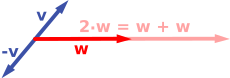
The first example of a vector space consists of arrows in a fixed plane, starting at one fixed point. This is used in physics to describe forces or velocities. Given any two such arrows, $v$ and $w$ , the parallelogram spanned by these two arrows contains one diagonal arrow that starts at the origin, too. This new arrow is called the sum of the two arrows, and is denoted $v + w$ . In the special case of two arrows on the same line, their sum is the arrow on this line whose length is the sum or the difference of the lengths, depending on whether the arrows have the same direction. Another operation that can be done with arrows is scaling: given any positive real number $a$ , the arrow that has the same direction as $v$ , but is dilated or shrunk by multiplying its length by $a$ , is called multiplication of $v$ by $a$ . It is denoted $a v$ . When $a$ is negative, $a v$ is defined as the arrow pointing in the opposite direction instead.

The following shows a few examples: if $a = 2$ , the resulting vector $a w$ has the same direction as $w$ , but is stretched to the double length of $w$ (right image below). Equivalently, $2 w$ is the sum $w + w$ . Moreover, $(-1) v = - v$ has the opposite direction and the same length as $v$ (blue vector pointing down in the right image).

Second example: ordered pairs of numbers[]

A second key example of a vector space is provided by pairs of real numbers $x$ and $y$ . (The order of the components $x$ and $y$ is significant, so such a pair is also called an ordered pair.) Such a pair is written as $(x, y)$ . The sum of two such pairs and multiplication of a pair with a number is defined as follows:

(x_{1},y_{1})+(x_{2},y_{2})=(x_{1}+x_{2},y_{1}+y_{2})

and

a(x,y)=(ax,ay).

The first example above reduces to this example, if an arrow is represented by a pair of Cartesian coordinates of its endpoint.

Notation and definition[]

In this article, vectors are represented in boldface to distinguish them from scalars.^{[nb 1]}

A vector space over a field $F$ is a set $V$ together with two operations that satisfy the eight axioms listed below. In the following, $V \times V$ denotes the Cartesian product of $V$ with itself, and $\to$ denotes a mapping from one set to another.

The first operation, called vector addition or simply addition $+ : V \times V \to V$ , takes any two vectors $v$ and $w$ and assigns to them a third vector which is commonly written as $v + w$ , and called the sum of these two vectors. (The resultant vector is also an element of the set $V$ .)
The second operation, called scalar multiplication $\cdot : F \times V \to V$ ， takes any scalar $a$ and any vector $v$ and gives another vector $a v$ . (Similarly, the vector $a v$ is an element of the set $V$ . Scalar multiplication is not to be confused with the scalar product, also called inner product or dot product, which is an additional structure present on some specific, but not all vector spaces. Scalar multiplication is a multiplication of a vector by a scalar; the other is a multiplication of two vectors producing a scalar.)

Elements of $V$ are commonly called vectors. Elements of $F$ are commonly called scalars. Common symbols for denoting vector spaces include $U$ , $V$ , and $W$ .

In the two examples above, the field is the field of the real numbers, and the set of the vectors consists of the planar arrows with a fixed starting point and pairs of real numbers, respectively.

To qualify as a vector space, the set $V$ and the operations of vector addition and scalar multiplication must adhere to a number of requirements called axioms.^[1] These are listed in the table below, where $u$ , $v$ and $w$ denote arbitrary vectors in $V$ , and $a$ and $b$ denote scalars in $F$ .^[2]^[3]

Axiom	Meaning
Associativity of vector addition	$u + (v + w) = (u + v) + w$
Commutativity of vector addition	$u + v = v + u$
Identity element of vector addition	There exists an element $0 \in V$ , called the zero vector, such that $v + 0 = v$ for all $v \in V$ .
Inverse elements of vector addition	For every $v \in V$ , there exists an element $- v \in V$ , called the additive inverse of $v$ , such that $v + (- v) = 0$ .
Compatibility of scalar multiplication with field multiplication	$a (b v) = (ab) v$ ^{[nb 2]}
Identity element of scalar multiplication	$1 v = v$ , where $1$ denotes the multiplicative identity in $F$ .
Distributivity of scalar multiplication with respect to vector addition	$a (u + v) = a u + a v$
Distributivity of scalar multiplication with respect to field addition	$(a + b) v = a v + b v$

These axioms generalize properties of the vectors introduced in the above examples. Indeed, the result of addition of two ordered pairs (as in the second example above) does not depend on the order of the summands:

(x v, y v) + (x w, y w) = (x w, y w) + (x v, y v)

.

Likewise, in the geometric example of vectors as arrows, $v + w = w + v$ since the parallelogram defining the sum of the vectors is independent of the order of the vectors. All other axioms can be verified in a similar manner in both examples. Thus, by disregarding the concrete nature of the particular type of vectors, the definition incorporates these two and many more examples in one notion of vector space.

Subtraction of two vectors and division by a (non-zero) scalar can be defined as

{\begin{aligned}\mathbf {v} -\mathbf {w} &=\mathbf {v} +(-\mathbf {w} )\\{\frac {\mathbf {v} }{a}}&={\frac {1}{a}}\mathbf {v} .\end{aligned}}

When the scalar field $F$ is the real numbers $R$ , the vector space is called a real vector space. When the scalar field is the complex numbers $C$ , the vector space is called a complex vector space. These two cases are the ones used most often in engineering. The general definition of a vector space allows scalars to be elements of any fixed field $F$ . The notion is then known as an $F$ -vector space or a vector space over $F$ . A field is, essentially, a set of numbers possessing addition, subtraction, multiplication and division operations.^{[nb 3]} For example, rational numbers form a field.

In contrast to the intuition stemming from vectors in the plane and higher-dimensional cases, in general vector spaces, there is no notion of nearness, angles or distances. To deal with such matters, particular types of vector spaces are introduced; see § Vector spaces with additional structure below for more.

Alternative formulations and elementary consequences[]

Vector addition and scalar multiplication are operations, satisfying the closure property: $u + v$ and $a v$ are in $V$ for all $a$ in $F$ , and $u$ , $v$ in $V$ . Some older sources mention these properties as separate axioms.^[4]

In the parlance of abstract algebra, the first four axioms are equivalent to requiring the set of vectors to be an abelian group under addition. The remaining axioms give this group an $F$ -module structure. In other words, there is a ring homomorphism $f$ from the field $F$ into the endomorphism ring of the group of vectors. Then scalar multiplication $a v$ is defined as $(f (a))(v)$ .^[5]

There are a number of direct consequences of the vector space axioms. Some of them derive from elementary group theory, applied to the additive group of vectors: for example, the zero vector $0$ of $V$ and the additive inverse $- v$ of any vector $v$ are unique. Further properties follow by employing also the distributive law for the scalar multiplication, for example $a v$ equals $0$ if and only if $a$ equals $0$ or $v$ equals $0$ .

History[]

Vector spaces stem from affine geometry, via the introduction of coordinates in the plane or three-dimensional space. Around 1636, French mathematicians René Descartes and Pierre de Fermat founded analytic geometry by identifying solutions to an equation of two variables with points on a plane curve.^[6] To achieve geometric solutions without using coordinates, Bolzano introduced, in 1804, certain operations on points, lines and planes, which are predecessors of vectors.^[7] Möbius (1827) introduced the notion of barycentric coordinates. Bellavitis (1833) introduced the notion of a bipoint, i.e., an oriented segment one of whose ends is the origin and the other one a target.^[8] Vectors were reconsidered with the presentation of complex numbers by Argand and Hamilton and the inception of quaternions by the latter.^[9] They are elements in R² and R⁴; treating them using linear combinations goes back to Laguerre in 1867, who also defined systems of linear equations.

In 1857, Cayley introduced the matrix notation which allows for a harmonization and simplification of linear maps. Around the same time, Grassmann studied the barycentric calculus initiated by Möbius. He envisaged sets of abstract objects endowed with operations.^[10] In his work, the concepts of linear independence and dimension, as well as scalar products are present. Actually Grassmann's 1844 work exceeds the framework of vector spaces, since his considering multiplication, too, led him to what are today called algebras. Italian mathematician Peano was the first to give the modern definition of vector spaces and linear maps in 1888.^[11]

An important development of vector spaces is due to the construction of function spaces by Henri Lebesgue. This was later formalized by Banach and Hilbert, around 1920.^[12] At that time, algebra and the new field of functional analysis began to interact, notably with key concepts such as spaces of p-integrable functions and Hilbert spaces.^[13] Also at this time, the first studies concerning infinite-dimensional vector spaces were done.

Examples[]

Coordinate space[]

The simplest example of a vector space over a field $F$ is the field $F$ itself (as it is an abelian group for addition, a part of requirements to be a field.), equipped with its addition (It becomes vector addition.) and multiplication (It becomes scalar multiplication.). More generally, all $n$ -tuples (sequences of length $n$ )

(a 1, a 2, ..., a n)

of elements $a i$ of $F$ form a vector space that is usually denoted $F n$ and called a coordinate space.^[14] The case $n = 1$ is the above-mentioned simplest example, in which the field $F$ is also regarded as a vector space over itself. The case $F = R$ and $n = 2$ (so R²) was discussed in the introduction above.

Complex numbers and other field extensions[]

The set of complex numbers $C$ , that is, numbers that can be written in the form $x + iy$ for real numbers $x$ and $y$ where $i$ is the imaginary unit, form a vector space over the reals with the usual addition and multiplication: $(x + iy) + (a + ib) = (x + a) + i (y + b)$ and $c \cdot (x + iy) = (c \cdot x) + i (c \cdot y)$ for real numbers $x$ , $y$ , $a$ , $b$ and $c$ . The various axioms of a vector space follow from the fact that the same rules hold for complex number arithmetic.

In fact, the example of complex numbers is essentially the same as (that is, it is isomorphic to) the vector space of ordered pairs of real numbers mentioned above: if we think of the complex number $x + i y$ as representing the ordered pair $(x, y)$ in the complex plane then we see that the rules for addition and scalar multiplication correspond exactly to those in the earlier example.

More generally, field extensions provide another class of examples of vector spaces, particularly in algebra and algebraic number theory: a field $F$ containing a smaller field $E$ is an $E$ -vector space, by the given multiplication and addition operations of $F$ .^[15] For example, the complex numbers are a vector space over $R$ , and the field extension $\mathbf {Q} (i{\sqrt {5}})$ is a vector space over $Q$ .

Function spaces[]

Addition of functions: The sum of the sine and the exponential function is

\sin +\exp :\mathbb {R} \to \mathbb {R}

with

(\sin +\exp )(x)=\sin(x)+\exp(x)

Functions from any fixed set $Ω$ to a field $F$ also form vector spaces, by performing addition and scalar multiplication pointwise. That is, the sum of two functions $f$ and $g$ is the function $(f + g)$ given by

(f + g)(w) = f (w) + g (w)

,

and similarly for multiplication. Such function spaces occur in many geometric situations, when $Ω$ is the real line or an interval, or other subsets of $R$ . Many notions in topology and analysis, such as continuity, integrability or differentiability are well-behaved with respect to linearity: sums and scalar multiples of functions possessing such a property still have that property.^[16] Therefore, the set of such functions are vector spaces. They are studied in greater detail using the methods of functional analysis, see below.^{[clarification needed]} Algebraic constraints also yield vector spaces: the vector space $F [x]$ is given by polynomial functions:

f (x) = r 0 + r 1 x + ... + r n -1 x n -1 + r n x n

, where the coefficients

r 0, ..., r n

are in

F

.^[17]

Linear equations[]

Systems of homogeneous linear equations are closely tied to vector spaces.^[18] For example, the solutions of

$a$	$+$	$3 b$	$+$	$c$	$= 0$
$4 a$	$+$	$2 b$	$+$	$2 c$	$= 0$

are given by triples with arbitrary $a$ , $b = a /2$ , and $c = -5 a /2$ . They form a vector space: sums and scalar multiples of such triples still satisfy the same ratios of the three variables; thus they are solutions, too. Matrices can be used to condense multiple linear equations as above into one vector equation, namely

A x = 0

,

where $A={\begin{bmatrix}1&3&1\\4&2&2\end{bmatrix}}$ is the matrix containing the coefficients of the given equations, $x$ is the vector $(a, b, c)$ , $A x$ denotes the matrix product, and $0 = (0, 0)$ is the zero vector. In a similar vein, the solutions of homogeneous linear differential equations form vector spaces. For example,

f''(x) + 2 f'(x) + f (x) = 0

yields $f (x) = a e - x + bx e - x$ , where $a$ and $b$ are arbitrary constants, and $e x$ is the natural exponential function.

Basis and dimension[]

A vector

v

in

R 2

(blue) expressed in terms of different bases: using the standard basis of

R 2

:

v = x e 1 + y e 2

(black), and using a different, non-orthogonal basis:

v = f 1 + f 2

(red).

Bases allow one to represent vectors by a sequence of scalars called coordinates or components. A basis is a set $B = {b i} i \in I$ of vectors $b i$ , for convenience often indexed by some index set $I$ , that spans the whole space and is linearly independent. "Spanning the whole space" means that any vector $v$ can be expressed as a finite sum (called a linear combination) of the basis elements:

\mathbf {v} =a_{1}\mathbf {b} _{i_{1}}+a_{2}\mathbf {b} _{i_{2}}+\cdots +a_{n}\mathbf {b} _{i_{n}},

(1)

where the $a k$ are scalars, called the coordinates (or the components) of the vector $v$ with respect to the basis $B$ , and $b i k$ $(k = 1, ..., n)$ elements of $B$ . Linear independence means that the coordinates $a k$ are uniquely determined for any vector in the vector space.

For example, the coordinate vectors $e 1 = (1, 0, \dots, 0)$ , $e 2 = (0, 1, 0, \dots, 0)$ , to $e n = (0, 0, \dots, 0, 1)$ , form a basis of $F n$ , called the standard basis, since any vector $(x 1, x 2, \dots, x n)$ can be uniquely expressed as a linear combination of these vectors:

(x 1, x 2, \dots, x n) = x 1 (1, 0, \dots, 0) + x 2 (0, 1, 0, \dots, 0) + \dots + x n (0, \dots, 0, 1) = x 1 e 1 + x 2 e 2 + \dots + x n e n

.

The corresponding coordinates $x 1$ , $x 2$ , $\dots$ , $x n$ are just the Cartesian coordinates of the vector.

Every vector space has a basis. This follows from Zorn's lemma, an equivalent formulation of the Axiom of Choice.^[19] Given the other axioms of Zermelo–Fraenkel set theory, the existence of bases is equivalent to the axiom of choice.^[20] The ultrafilter lemma, which is weaker than the axiom of choice, implies that all bases of a given vector space have the same number of elements, or cardinality (cf. Dimension theorem for vector spaces).^[21] It is called the dimension of the vector space, denoted by dim V. If the space is spanned by finitely many vectors, the above statements can be proven without such fundamental input from set theory.^[22]

The dimension of the coordinate space $F n$ is $n$ , by the basis exhibited above. The dimension of the polynomial ring F[x] introduced above^{[clarification needed]} is countably infinite, a basis is given by $1$ , $x$ , $x 2$ , $\dots$ A fortiori, the dimension of more general function spaces, such as the space of functions on some (bounded or unbounded) interval, is infinite.^{[nb 4]} Under suitable regularity assumptions on the coefficients involved, the dimension of the solution space of a homogeneous ordinary differential equation equals the degree of the equation.^[23] For example, the solution space for the above equation^{[clarification needed]} is generated by $e - x and xe - x$ . These two functions are linearly independent over $R$ , so the dimension of this space is two, as is the degree of the equation.

A field extension over the rationals $Q$ can be thought of as a vector space over $Q$ (by defining vector addition as field addition, defining scalar multiplication as field multiplication by elements of $Q$ , and otherwise ignoring the field multiplication). The dimension (or degree) of the field extension $Q (α)$ over $Q$ depends on $α$ . If $α$ satisfies some polynomial equation

q_{n}\alpha ^{n}+q_{n-1}\alpha ^{n-1}+\cdots +q_{0}=0

with rational coefficients

q n, ..., q 0

(in other words, if α is algebraic), the dimension is finite. More precisely, it equals the degree of the minimal polynomial having α as a root.^[24] For example, the complex numbers C are a two-dimensional real vector space, generated by 1 and the imaginary unit i. The latter satisfies i² + 1 = 0, an equation of degree two. Thus, C is a two-dimensional R-vector space (and, as any field, one-dimensional as a vector space over itself, C). If α is not algebraic, the dimension of Q(α) over Q is infinite. For example, for α = π there is no such equation. That is, π is transcendental.^[25]

Linear maps and matrices[]

The relation of two vector spaces can be expressed by linear map or linear transformation. They are functions that reflect the vector space structure, that is, they preserve sums and scalar multiplication:

f(\mathbf {v} +\mathbf {w} )=f(\mathbf {v} )+f(\mathbf {w} )

and

f (a \cdot v) = a \cdot f (v)

for all

v

and

w

in

V

, all

a

in

F

.^[26]

An isomorphism is a linear map $f : V \to W$ such that there exists an inverse map $g : W \to V$ , which is a map such that the two possible compositions $f \circ g : W \to W$ and $g \circ f : V \to V$ are identity maps. Equivalently, $f$ is both one-to-one (injective) and onto (surjective).^[27] If there exists an isomorphism between $V$ and $W$ , the two spaces are said to be isomorphic; they are then essentially identical as vector spaces, since all identities holding in $V$ are, via $f$ , transported to similar ones in $W$ , and vice versa via $g$ .

Describing an arrow vector

v

by its coordinates

x

and

y

yields an isomorphism of vector spaces.

For example, the "arrows in the plane" and "ordered pairs of numbers" vector spaces in the introduction are isomorphic: a planar arrow $v$ departing at the origin of some (fixed) coordinate system can be expressed as an ordered pair by considering the $x$ - and $y$ -component of the arrow, as shown in the image at the right. Conversely, given a pair $(x, y)$ , the arrow going by $x$ to the right (or to the left, if $x$ is negative), and $y$ up (down, if $y$ is negative) turns back the arrow $v$ .

Linear maps $V \to W$ between two vector spaces form a vector space $Hom F (V, W)$ , also denoted $L(V, W)$ , or

[nb 1]

[1]

[2]

[3]

[nb 2]

[nb 3]

[4]

[5]

[6]

[7]

[8]

[9]

[10]

[11]

[12]

[13]

[14]

[15]

[16]

[17]

[18]

[19]

[20]

[21]

[22]

[nb 4]

[23]

[24]

[25]

[26]

[27]