Azimuthal quantum number

The atomic orbital wavefunctions of a hydrogen atom. The principal quantum number (n) is at the right of each row and the azimuthal quantum number (ℓ) is denoted by letter at top of each column.

Part of a series of articles about
Quantum mechanics
${\displaystyle i\hbar {\frac {\partial }{\partial t}}|\psi (t)\rangle ={\hat {H}}|\psi (t)\rangle }$ Schrödinger equation
Introduction Glossary History
Background Classical mechanics Old quantum theory Bra–ket notation Hamiltonian Interference
Fundamentals Complementarity Decoherence Entanglement Energy level Measurement Nonlocality Quantum number State Superposition Symmetry Tunnelling Uncertainty Wave function Collapse
Experiments Bell's inequality Davisson–Germer Double-slit Elitzur–Vaidman Franck–Hertz Leggett–Garg inequality Mach–Zehnder Popper Quantum eraser Delayed-choice Schrödinger's cat Stern–Gerlach Wheeler's delayed-choice
Formulations Overview Heisenberg Interaction Matrix Phase-space Schrödinger Sum-over-histories (path integral)
Equations Dirac Klein–Gordon Pauli Rydberg Schrödinger
Interpretations Overview Bayesian Consistent histories Copenhagen de Broglie–Bohm Ensemble Hidden-variable Local Many-worlds Objective collapse Quantum logic Relational Transactional
Advanced topics Relativistic quantum mechanics Quantum field theory Quantum information science Quantum computing Quantum chaos Density matrix Scattering theory Quantum statistical mechanics Quantum machine learning
Scientists Aharonov Bell Bethe Blackett Bloch Bohm Bohr Born Bose de Broglie Compton Dirac Davisson Debye Ehrenfest Einstein Everett Fock Fermi Feynman Glauber Gutzwiller Heisenberg Hilbert Jordan Kramers Pauli Lamb Landau Laue Moseley Millikan Onnes Planck Rabi Raman Rydberg Schrödinger Simmons Sommerfeld von Neumann Weyl Wien Wigner Zeeman Zeilinger
v t

The azimuthal quantum number is a quantum number for an atomic orbital that determines its orbital angular momentum and describes the shape of the orbital. The azimuthal quantum number is the second of a set of quantum numbers that describe the unique quantum state of an electron (the others being the principal quantum number, the magnetic quantum number, and the spin quantum number). It is also known as the orbital angular momentum quantum number, orbital quantum number or second quantum number, and is symbolized as ℓ (pronounced ell).

Derivation[]

Connected with the energy states of the atom's electrons are four quantum numbers: n, ℓ, m_ℓ, and m_s. These specify the complete, unique quantum state of a single electron in an atom, and make up its wavefunction or orbital. When solving to obtain the wave function, the Schrödinger equation reduces to three equations that lead to the first three quantum numbers. Therefore, the equations for the first three quantum numbers are all interrelated. The azimuthal quantum number arose in the solution of the polar part of the wave equation as shown below^[where?], reliant on the spherical coordinate system, which generally works best with models having some glimpse of spherical symmetry.

Illustration of quantum mechanical orbital angular momentum.

An atomic electron's angular momentum, L, is related to its quantum number ℓ by the following equation:

${\displaystyle \mathbf {L} ^{2}\Psi =\hbar ^{2}\ell (\ell +1)\Psi ,}$

where ħ is the reduced Planck's constant, L² is the orbital angular momentum operator and ${\displaystyle \Psi }$ is the wavefunction of the electron. The quantum number ℓ is always a non-negative integer: 0, 1, 2, 3, etc. L has no real meaning except in its use as the angular momentum operator. When referring to angular momentum, it is better to simply use the quantum number ℓ.

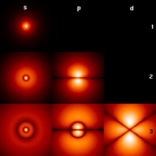
Atomic orbitals have distinctive shapes denoted by letters. In the illustration, the letters s, p, and d (a convention originating in spectroscopy) describe the shape of the atomic orbital.

Their wavefunctions take the form of spherical harmonics, and so are described by Legendre polynomials. The various orbitals relating to different values of ℓ are sometimes called sub-shells, and are referred to by lowercase Latin letters (chosen for historical reasons), as follows:

Quantum subshells for the azimuthal quantum number

Azimuthal number (ℓ)	Historical letter	Maximum electrons	Historical name	Shape
0	s	2	sharp	spherical
1	p	6	principal	three dumbbell-shaped polar-aligned orbitals; one lobe on each pole of the x, y, and z (+ and − axes)
2	d	10	diffuse	nine dumbbells and one doughnut (or “unique shape #1” see this picture of spherical harmonics, third row center)
3	f	14	fundamental	“unique shape #2” (see this picture of spherical harmonics, bottom row center)
4	g	18
5	h	22
6	i	26
The letters after the f sub-shell just follow letter f in alphabetical order, except the letter j and those already used.

Each of the different angular momentum states can take 2(2ℓ + 1) electrons. This is because the third quantum number m_ℓ (which can be thought of loosely as the quantized projection of the angular momentum vector on the z-axis) runs from −ℓ to ℓ in integer units, and so there are 2ℓ + 1 possible states. Each distinct n, ℓ, m_ℓ orbital can be occupied by two electrons with opposing spins (given by the quantum number m_s = ±½), giving 2(2ℓ + 1) electrons overall. Orbitals with higher ℓ than given in the table are perfectly permissible, but these values cover all atoms so far discovered.

For a given value of the principal quantum number n, the possible values of ℓ range from 0 to n − 1; therefore, the n = 1 shell only possesses an s subshell and can only take 2 electrons, the n = 2 shell possesses an s and a p subshell and can take 8 electrons overall, the n = 3 shell possesses s, p, and d subshells and has a maximum of 18 electrons, and so on.

A simplistic one-electron model results in energy levels depending on the principal number alone. In more complex atoms these energy levels split for all n > 1, placing states of higher ℓ above states of lower ℓ. For example, the energy of 2p is higher than of 2s, 3d occurs higher than 3p, which in turn is above 3s, etc. This effect eventually forms the block structure of the periodic table. No known atom possesses an electron having ℓ higher than three (f) in its ground state.

The angular momentum quantum number, ℓ, governs^[how?] the number of planar nodes going through the nucleus. A planar node can be described in an electromagnetic wave as the midpoint between crest and trough, which has zero magnitudes. In an s orbital, no nodes go through the nucleus, therefore the corresponding azimuthal quantum number ℓ takes the value of 0. In a p orbital, one node traverses the nucleus and therefore ℓ has the value of 1. ${\displaystyle L}$ has the value ${\displaystyle {\sqrt {2}}\hbar }$.

Depending on the value of n, there is an angular momentum quantum number ℓ and the following series. The wavelengths listed are for a hydrogen atom:

${\displaystyle n=1,L=0}$, Lyman series (ultraviolet)

${\displaystyle n=2,L={\sqrt {2}}\hbar }$, Balmer series (visible)

${\displaystyle n=3,L={\sqrt {6}}\hbar }$, Ritz–Paschen series (near infrared)

${\displaystyle n=4,L=2{\sqrt {3}}\hbar }$, Brackett series (short-wavelength infrared)

${\displaystyle n=5,L=2{\sqrt {5}}\hbar }$, Pfund series (mid-wavelength infrared).

Addition of quantized angular momenta[]

Given a quantized total angular momentum ${\displaystyle {\vec {\jmath }}}$ which is the sum of two individual quantized angular momenta ${\displaystyle {\vec {\ell _{1}}}}$ and ${\displaystyle {\vec {\ell _{2}}}}$,

${\displaystyle {\vec {\jmath }}={\vec {\ell _{1}}}+{\vec {\ell _{2}}}}$

the quantum number ${\displaystyle j}$ associated with its magnitude can range from ${\displaystyle |\ell _{1}-\ell _{2}|}$ to ${\displaystyle \ell _{1}+\ell _{2}}$ in integer steps where ${\displaystyle \ell _{1}}$ and ${\displaystyle \ell _{2}}$ are quantum numbers corresponding to the magnitudes of the individual angular momenta.

Total angular momentum of an electron in the atom[]

"Vector cones" of total angular momentum J (purple), orbital L (blue), and spin S (green). The cones arise due to quantum uncertainty between measuring angular momentum components (see ).

Due to the spin–orbit interaction in the atom, the orbital angular momentum no longer commutes with the Hamiltonian, nor does the spin. These therefore change over time. However the total angular momentum J does commute with the one-electron Hamiltonian and so is constant. J is defined through

${\displaystyle {\vec {J}}={\vec {L}}+{\vec {S}}}$

L being the orbital angular momentum and S the spin. The total angular momentum satisfies the same commutation relations as orbital angular momentum, namely

${\displaystyle [J_{i},J_{j}]=i\hbar \epsilon _{ijk}J_{k}}$

from which follows

${\displaystyle \left[J_{i},J^{2}\right]=0}$

where J_i stand for J_x, J_y, and J_z.

The quantum numbers describing the system, which are constant over time, are now j and m_j, defined through the action of J on the wavefunction ${\displaystyle \Psi }$

${\displaystyle \mathbf {J} ^{2}\Psi =\hbar ^{2}{j(j+1)}\Psi }$

${\displaystyle \mathbf {J} _{z}\Psi =\hbar {m_{j}}\Psi }$

So that j is related to the norm of the total angular momentum and m_j to its projection along a specified axis. The j number has a particular importance for relativistic quantum chemistry, often featuring in subscript in electron configuration of superheavy elements.

As with any angular momentum in quantum mechanics, the projection of J along other axes cannot be co-defined with J_z, because they do not commute.

Relation between new and old quantum numbers[]

j and m_j, together with the parity of the quantum state, replace the three quantum numbers ℓ, m_ℓ and m_s (the projection of the spin along the specified axis). The former quantum numbers can be related to the latter.

Furthermore, the eigenvectors of j, s, m_j and parity, which are also eigenvectors of the Hamiltonian, are linear combinations of the eigenvectors of ℓ, s, m_ℓ and m_s.

List of angular momentum quantum numbers[]

• Intrinsic (or spin) angular momentum quantum number, or simply spin quantum number
• orbital angular momentum quantum number (the subject of this article)
• magnetic quantum number, related to the orbital momentum quantum number
• total angular momentum quantum number

History[]

The azimuthal quantum number was carried over from the Bohr model of the atom, and was posited by Arnold Sommerfeld.^[1] The Bohr model was derived from spectroscopic analysis of the atom in combination with the Rutherford atomic model. The lowest quantum level was found to have an angular momentum of zero. Orbits with zero angular momentum were considered as oscillating charges in one dimension and so described as "pendulum" orbits, but were not found in nature.^[2] In three-dimensions the orbits become spherical without any nodes crossing the nucleus, similar (in the lowest-energy state) to a skipping rope that oscillates in one large circle.

See also[]

• Angular momentum operator
• Introduction to quantum mechanics
• Particle in a spherically symmetric potential
• Angular momentum coupling
• Clebsch–Gordan coefficients

References[]

External links[]

• Development of the Bohr atom

• Detailed explanation of the Orbital Quantum Number l
• The azimuthal equation explained