Carrying capacity

The carrying capacity of an environment is the maximum population size of a biological species that can be sustained by that specific environment, given the food, habitat, water, and other resources available. The carrying capacity is defined as the environment's maximal load, which in population ecology corresponds to the population equilibrium, when the number of deaths in a population equals the number of births (as well as immigration and emigration). The effect of carrying capacity on population dynamics is modelled with a logistic function. Carrying capacity is applied to the maximum population an environment can support in ecology, agriculture and fisheries. The term carrying capacity has been applied to a few different processes in the past before finally being applied to population limits in the 1950s.^[1] The notion of carrying capacity for humans is covered by the notion of sustainable population.

Origins[]

In terms of population dynamics, the term 'carrying capacity' was not explicitly used in 1838 by the Belgian mathematician Pierre François Verhulst when he first published his equations based on research on modelling population growth.^[2]

The origins of the term "carrying capacity" are uncertain, with sources variously stating that it was originally used "in the context of international shipping" in the 1840s,^[3][4] or that it was first used during 19th-century laboratory experiments with micro-organisms.^[5] A 2008 review finds the first use of the term in English was an 1845 report by the US Secretary of State to the US Senate. It then became a term used generally in biology in the 1870s, being most developed in wildlife and livestock management in the early 1900s.^[4] It had become a staple term in ecology used to define the biological limits of a natural system related to population size in the 1950s.^[3][4]

Neo-Malthusians and eugenicists popularised the use of the words to describe the number of people the Earth can support in the 1950s,^[4] although American biostatisticians Raymond Pearl and Lowell Reed had already applied it in these terms to human populations in the 1920s.^{[citation needed]}

Hadwen and Palmer (1922) defined carrying capacity as the density of stock that could be grazed for a definite period without damage to the range.^[6][7]

It was first used in the context of wildlife management by the American Aldo Leopold in 1933, and a year later by the also American , a wetlands specialist. Both used the term in different ways, Leopold largely in the sense of grazing animals (differentiating between a 'saturation level', an intrinsic level of density a species would live in, and carrying capacity, the most animals which could be in the field) and Errington defining 'carrying capacity' as the number of animals above which predation would become 'heavy' (this definition has largely been rejected, including by Errington himself).^[6][8] The important and popular 1953 textbook on ecology by Eugene Odum, Fundamentals of Ecology, popularised the term in its modern meaning as the equilibrium value of the logistic model of population growth.^[6][9]

Mathematics[]

The specific reason why a population stops growing is known as a limiting or regulating factor.^{[citation needed]}

Reaching carrying capacity through a logistic growth curve

The difference between the birth rate and the death rate is the natural increase. If the population of a given organism is below the carrying capacity of a given environment, this environment could support a positive natural increase; should it find itself above that threshold the population typically decreases.^[10] Thus, the carrying capacity is the maximum number of individuals of a species that an environment can support.^[11]

Population size decreases above carrying capacity due to a range of factors depending on the species concerned, but can include insufficient space, food supply, or sunlight. The carrying capacity of an environment may vary for different species.^{[citation needed]}

In the standard ecological algebra as illustrated in the simplified Verhulst model of population dynamics, carrying capacity is represented by the constant K:

${\displaystyle {\frac {dN}{dt}}=rN\left(1-{\frac {N}{K}}\right)}$

where

N is the population size,

r is the intrinsic growth rate

K is the carrying capacity of the local environment, and

dN/dt, the derivative of N with respect to time t, is the rate of change in population with time.

Thus, the equation relates the growth rate of the population N to the current population size, incorporating the effect of the two constant parameters r and K. (Note that decrease is negative growth.) The choice of the letter K came from the German Kapazitätsgrenze (capacity limit).

This equation is a modification of the original Verhulst model:

${\displaystyle {\frac {dN}{dt}}=rN-\alpha N^{2}}$^[12]

In this equation, the carrying capacity K, ${\displaystyle N^{*}}$, is

${\displaystyle N^{*}={\frac {r}{\alpha }}.}$

This is a graph of the population due to the logistic curve model. When the population is above the carrying capacity it decreases, and when it is below the carrying capacity it increases.

When the Verhulst model is plotted into a graph, the population change over time takes the form of a sigmoid curve, reaching its highest level at K. This is the logistic growth curve and it is calculated with:

${\displaystyle f(x)={\frac {L}{1+e^{-k(x-x_{0})}}},}$

where

e is the natural logarithm base (also known as Euler's number),

x₀ is the x value of the sigmoid's midpoint,

L is the curve's maximum value,

K is the logistic growth rate or steepness of the curve ^[13] and

${\displaystyle f(x_{0})=L/2.}$

The logistic growth curve depicts how population growth rate and the carrying capacity are inter-connected. As illustrated in the logistic growth curve model, when the population size is small, the population increases exponentially. However, as population size nears the carrying capacity, the growth decreases and reaches zero at K.^[14]

What determines a specific system's carrying capacity involves a limiting factor which may be something such as available supplies of food, water, nesting areas, space or amount of waste that can be absorbed. Where resources are finite, such as for a population of Osedax on a whale fall or bacteria in a petridish, the population will curve back down to zero after the resources have been exhausted, with the curve reaching its apogee at K. In systems in which resources are constantly replenished, the population will reach its equilibrium at K.^{[citation needed]}

Software is available to help calculate the carrying capacity of a given natural environment.^[15]

Population ecology[]

Carrying capacity is a commonly used method for biologists when trying to better understand biological populations and the factors which affect them.^[1] When addressing biological populations, carrying capacity can be used as a stable dynamic equilibrium, taking into account extinction and colonization rates.^[10] In population biology, logistic growth assumes that population size fluctuates above and below an equilibrium value.^[16]

Numerous authors have questioned the usefulness of the term when applied to actual wild populations.^[6][7][17] Although useful in theory and in laboratory experiments, the use of carrying capacity as a method of measuring population limits in the environment is less useful as it assumes no interactions between species.^[10]

Agriculture[]

Calculating the carrying capacity of a paddock in Australia is done in Dry Sheep Equivalents (DSEs). A single DSE is 50 kg Merino wether, dry ewe or non-pregnant ewe, which is maintained in a stable condition. Not only sheep are calculated in DSEs, the carrying capacity for other livestock is also calculated using this measure. A 200 kg weaned calf of a British style breed gaining 0.25 kg/day is 5.5DSE, but if the same weight of the same type of calf were gaining 0.75 kg/day, it would be measure at 8DSE. Cattle are not all the same, their DSEs can vary depending on breed, growth rates, weights, if it is a cow ('dam'), steer or ox ('bullock' in Australia), and if it weaning, pregnant or 'wet' (i.e. lactating). It is important for farmers to calculate the carrying capacity of their land so they can establish a sustainable stocking rate.^[18] In other parts of the world different units are used for calculating carrying capacities. In the United Kingdom the paddock is measured in LU, livestock units, although different schemes exist for this.^[19][20] New Zealand uses either LU,^[21] EE (ewe equivalents) or SU (stock units).^[22] In the USA and Canada the traditional system uses animal units (AU).^[23] A French/Swiss unit is Unité de Gros Bétail (UGB).^[24][25]

Summering of milk cows in the Swiss Alps in Valais Canton

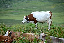
In some European countries such as Switzerland the pasture (alm or alp) is traditionally measured in Stoß, with one Stoß equalling four Füße (feet). A more modern European system is Großvieheinheit (GV or GVE), corresponding to 500 kg in liveweight of cattle. In extensive agriculture 2 GV/ha is a common stocking rate, in intensive agriculture, when grazing is supplemented with extra fodder, rates can be 5 to 10 GV/ha.^{[citation needed]} In Europe average stocking rates vary depending on the country, in 2000 the Netherlands and Belgium had a very rate of 3.82 GV/ha and 3.19 GV/ha respectively, surrounding countries have rates of around 1 to 1.5 GV/ha, and more southern European countries have lower rates, with Spain having the lowest rate of 0.44 GV/ha.^[26] This system can also be applied to natural areas. Grazing megaherbivores at roughly 1 GV/ha is considered sustainable in central European grasslands, although this varies widely depending on many factors. In ecology it is theoretically (i.e. cyclic succession, patch dynamics, Megaherbivorenhypothese) taken that a grazing pressure of 0.3 GV/ha by wildlife is enough to hinder afforestation in a natural area. Because different species have different ecological niches, with horses for example grazing short grass, cattle longer grass, and goats or deer preferring to browse shrubs, niche differentiation allows a terrain to have slightly higher carrying capacity for a mixed group of species, than it would if there were only one species involved.^{[citation needed]}

Some niche market schemes mandate lower stocking rates than can maximally be grazed on a pasture. In order to market ones' meat products as 'biodynamic', a lower Großvieheinheit of 1 to 1.5 (2.0) GV/ha is mandated, with some farms having an operating structure using only 0.5 to 0.8 GV/ha.^{[citation needed]}

The Food and Agriculture Organization has introduced three international units: FAO Livestock Units for North America,^[27][28] FAO Livestock Units for sub-Saharan Africa,^[27][28] and Tropical Livestock Units.^[29]

Another rougher and less precise method of determining the carrying capacity of a paddock is simply by looking objectively at the condition of the herd. In Australia, the national standardized system for rating livestock conditions is done by body condition scoring (BCS). An animal in a very poor condition is scored with a BCS of 0, and an animal which is extremely healthy is scored at 5: animals may be scored between these two numbers in increments of 0.25. At least 25 animals of the same type must be scored to provide a statistically representative number, and scoring must take place monthly -if the average falls, this may be due to a stocking rate above the paddock's carrying capacity or too little fodder. This method is less direct for determining stocking rates than looking at the pasture itself, because the changes in the condition of the stock may lag behind changes in the condition of the pasture.^[18]

Fisheries[]

A fishery at sunset in Cochin, Kerala, India.

In fisheries, the carrying capacity is used in the formulae to calculate sustainable yields for fisheries management.^[30] The maximum sustainable yield (MSY) is defined as "the highest average catch that can be continuously taken from an exploited population (=stock) under average environmental conditions". It was originally calculated as half of the carrying capacity, but has been refined over the years,^[31] now being seen as roughly 30% of the population, depending on the species or population.^[32][33] Because the population of a species which is brought below its carrying capacity due to fishing will find itself in the exponential phase of growth, as seen in the Verhulst model, the harvesting of an amount of fish at or below MSY is a surplus yield which can be sustainably harvested without reducing population size at equilibrium, keeping the population at its maximum recruitment (however, annual fishing can be seen as a modification of r in the equation -i.e. the environment has been modified, which means that the population size at equilibrium with annual fishing is slightly below what K would be without it). Note that mathematically and in practical terms, MSY is problematic. If mistakes are made and even a tiny amount of fish are harvested each year above the MSY, populations dynamics imply that the total population will eventually decrease to zero. The actual carrying capacity of the environment may fluctuate in the real world, which means that practically, MSY may actually vary slightly from year to year^[34][35][36] (annual sustainable yields and maximum average yield attempt to take this into account).^{[citation needed]} Other similar concepts are optimum sustainable yield and , these are both harvest rates below MSY.^[37][38]

These calculations are used to determine fishing quotas.^{[citation needed]}

See also[]

References[]