Hunting oscillation

Hunting oscillation is a self-oscillation, usually unwanted, about an equilibrium.[1] The expression came into use in the 19th century and describes how a system "hunts" for equilibrium.[1] The expression is used to describe phenomena in such diverse fields as electronics, aviation, biology, and railway engineering.[1]
Railway wheelsets[]
A classical hunting oscillation is a swaying motion of a railway vehicle (often called truck hunting or bogie hunting) caused by the coning action on which the directional stability of an adhesion railway depends. It arises from the interaction of adhesion forces and inertial forces. At low speed, adhesion dominates but, as the speed increases, the adhesion forces and inertial forces become comparable in magnitude and the oscillation begins at a critical speed. Above this speed, the motion can be violent, damaging track and wheels and potentially causing derailment. The problem does not occur on systems with a differential because the action depends on both wheels of a wheelset rotating at the same angular rate, although differentials tend to be rare, and conventional trains have their wheels fixed to the axles in pairs instead. Some trains, like the Talgo 350, have no differential, yet they are mostly not affected by hunting oscillation, as most of their wheels rotate independently from one another. The wheels of the power car, however, can be affected by hunting oscillation, because the wheels of the power car are fixed to the axles in pairs like in conventional bogies. Less conical wheels and bogies equipped with independent wheels that turn independently from each other and are not fixed to an axle in pairs are cheaper than a suitable differential for the bogies of a train.[2]
The problem was first noticed towards the end of the 19th century, when train speeds became high enough to encounter it. Serious efforts to counteract it got underway in the 1930s, giving rise to lengthened trucks and the side-damping swing hanger truck. In the development of the Japanese Shinkansen, less-conical wheels and other design changes were used to extend truck design speeds above 225 km/h (140 mph). Advances in wheel and truck design based on research and development efforts in Europe and Japan have extended the speeds of steel wheel systems well beyond those attained by the original Shinkansen, while the advantage of backwards compatibility keeps such technology dominant over alternatives such as the hovertrain and maglev systems. The speed record for steel-wheeled trains is held by the French TGV, at 574.9 km/h (357 mph).
Kinematic analysis[]
While a qualitative description provides some understanding of the phenomenon, deeper understanding inevitably requires a mathematical analysis of the vehicle dynamics. Even then, the results may be only approximate.
A kinematic description deals with the geometry of motion, without reference to the forces causing it, so the analysis begins with a description of the geometry of a wheel set running on a straight track. Since Newton's second law relates forces to the acceleration of bodies, the forces acting may then be derived from the kinematics by calculating the accelerations of the components. However, if these forces change the kinematic description (as they do in this case) then the results may only be approximately correct.
Assumptions and non-mathematical description[]
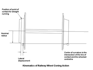
This kinematic description makes a number of simplifying assumptions since it neglects forces. For one, it assumes that the rolling resistance is zero. A wheelset (not attached to a train or truck), is given a push forward on a straight and level track. The wheelset starts coasting and never slows down since there are no forces (except downward forces on the wheelset to make it adhere to the track and not slip). If initially the wheelset is centered on the railroad track then the effective diameters of each wheel are the same and the wheelset rolls down the track in a perfectly straight line forever. But if the wheelset is a little off-center so that the effective diameters (or radii) are different, then the wheelset starts to move in a curve of radius R (depending on these wheelset radii, etc.; to be derived later on). The problem is to use kinematic reasoning to find the trajectory of the wheelset, or more precisely, the trajectory of the center of the wheelset projected vertically on the roadbed in the center of the track. This is a trajectory on the plane of the level earth's surface and plotted on an x-y graphical plot where x is the distance along the railroad and y is the "tracking error", the deviation of the center of the wheelset from the straight line of the railway running down the center of the track (midway between the two rails).
To illustrate that a wheelset trajectory follows a curved path, one may place a nail or screw on a flat table top and give it a push. It will roll in a circular curve because the nail or screw is like a wheelset with extremely different diameter wheels. The head is analogous to a large diameter wheel and the pointed end is like a small diameter wheel. While the nail or screw will turn around in a full circle (and more) the railroad wheelset behaves differently because as soon at it starts to turn in a curve, the effective diameters change in such a way as to decrease the curvature of the path. Note that "radius" and "curvature" refer to the curvature of the trajectory of the wheelset and not the curvature of the railway since this is perfectly straight track. As the wheelset rolls on, the curvature decreases until the wheels reach the point where their effective diameters are equal and the path is no longer curving. But the trajectory has a slope at this point (it is a straight line which crosses diagonally over the centerline of the track) so that it overshoots the centerline of the track and the effective diameters reverse (the formerly smaller diameter wheel becomes the larger diameter and conversely). This results in the wheelset moving in a curve in the opposite direction. Again it overshoots the centerline and this phenomenon continues indefinitely with the wheelset oscillating from side to side. Note that the wheel flange never makes contact with the rail. In this model, the rails are assumed to always contact the wheel tread along the same line on the rail head which assumes that the rails are knife-edge and only make contact with the wheel tread along a line (of zero width).
Mathematical analysis[]
The train stays on the track by virtue of the conical shape of the wheel treads. If a wheelset is displaced to one side by an amount y (the tracking error), the radius of the tread in contact with the rail on one side is reduced, while on the other side it is increased. The angular velocity is the same for both wheels (they are coupled via a rigid axle), so the larger diameter tread speeds up, while the smaller slows down. The wheel set steers around a centre of curvature defined by the intersection of the generator of a cone passing through the points of contact with the wheels on the rails and the axis of the wheel set. Applying similar triangles, we have for the turn radius:
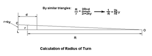

where d is the track gauge, r the wheel radius when running straight and k is the tread taper (which is the slope of tread in the horizontal direction perpendicular to the track).
The path of the wheel set relative to the straight track is defined by a function y(x), where x is the progress along the track. This is sometimes called the tracking error.[3] Provided the direction of motion remains more or less parallel to the rails, the curvature of the path may be related to the second derivative of y with respect to distance along the track as approximately[4]

It follows that the trajectory along the track is governed by the equation:[5]

This is a simple harmonic motion having wavelength:

This kinematic analysis implies that trains sway from side to side all the time. In fact, this oscillation is damped out below a critical speed and the ride is correspondingly more comfortable. The kinematic result ignores the forces causing the motion. These may be analyzed using the concept of creep (non-linear) but are somewhat difficult to quantify simply, as they arise from the elastic distortion of the wheel and rail at the regions of contact. These are the subject of frictional contact mechanics; an early presentation that includes these effects in hunting motion analysis was presented by Carter.[7] See Knothe[8] for a historical overview.
If the motion is substantially parallel with the rails, the angular displacement of the wheel set is given by:


Hence:

The angular deflection also follows a simple harmonic motion, which lags behind the side to side motion by a quarter of a cycle. In many systems which are characterised by harmonic motion involving two different states (in this case the axle yaw deflection and the lateral displacement), the quarter cycle lag between the two motions endows the system with the ability to extract energy from the forward motion. This effect is observed in "flutter" of aircraft wings and "shimmy" of road vehicles, as well as hunting of railway vehicles. The kinematic solution derived above describes the motion at the critical speed.
In practice, below the critical speed, the lag between the two motions is less than a quarter cycle so that the motion is damped out but, above the critical speed, the lag is greater than a quarter cycle so that the motion is amplified.
In order to estimate the inertial forces, it is necessary to express the distance derivatives as time derivatives. This is done using the speed of the vehicle U, which is assumed constant:

The angular acceleration of the axle in yaw is:

The inertial moment (ignoring gyroscopic effects) is:

where F is the force acting along the rails and C is the moment of inertia of the wheel set.

the maximum frictional force between the wheel and rail is given by:

where W is the axle load and is the coefficient of friction. Gross slipping will occur at a combination of speed and axle deflection given by:


this expression yields a significant overestimate of the critical speed, but it does illustrate the physical reason why hunting occurs, i.e. the inertial forces become comparable with the adhesion forces above a certain speed. Limiting friction is a poor representation of the adhesion force in this case.
The actual adhesion forces arise from the distortion of the tread and rail in the region of contact. There is no gross slippage, just elastic distortion and some local slipping (creep slippage). During normal operation these forces are well within the limiting friction constraint. A complete analysis takes these forces into account, using rolling contact mechanics theories.
However, the kinematic analysis assumed that there was no slippage at all at the wheel-rail contact. Now it is clear that there is some creep slippage which makes the calculated sinusoidal trajectory of the wheelset (per Klingel's formula) not exactly correct.
Energy balance[]
In order to get an estimate of the critical speed, we use the fact that the condition for which this kinematic solution is valid corresponds to the case where there is no net energy exchange with the surroundings, so by considering the kinetic and potential energy of the system, we should be able to derive the critical speed.
Let:

Using the operator:

the angular acceleration equation may be expressed in terms of the angular velocity in yaw, :


integrating:

so the kinetic energy due to rotation is:


When the axle yaws, the points of contact move outwards on the treads so that the height of the axle is lowered. The distance between the support points increases to:

(to second order of small quantities). the displacement of the support point out from the centres of the treads is:

the axle load falls by

The work done by lowering the axle load is therefore:

This is energy lost from the system, so in order for the motion to continue, an equal amount of energy must be extracted from the forward motion of the wheelset.
The outer wheel velocity is given by:

The kinetic energy is:

for the inner wheel it is

where m is the mass of both wheels.
The increase in kinetic energy is:

The motion will continue at constant amplitude as long as the energy extracted from the forward motion, and manifesting itself as increased kinetic energy of the wheel set at zero yaw, is equal to the potential energy lost by the lowering of the axle load at maximum yaw.
Now, from the kinematics:

but

The translational kinetic energy is

The total kinetic energy is:

The critical speed is found from the energy balance:

Hence the critical speed is given by

This is independent of the wheel taper, but depends on the ratio of the axle load to wheel set mass. If the treads were truly conical in shape, the critical speed would be independent of the taper. In practice, wear on the wheel causes the taper to vary across the tread width, so that the value of taper used to determine the potential energy is different from that used to calculate the kinetic energy. Denoting the former as a, the critical speed becomes:

where a is now a shape factor determined by the wheel wear. This result is derived in Wickens (1965)[9] from an analysis of the system dynamics using standard control engineering methods.
Limitation of simplified analysis[]
The motion of a wheel set is much more complicated than this analysis would indicate. There are additional restraining forces applied by the vehicle suspension[10] and, at high speed, the wheel set will generate additional gyroscopic torques, which will modify the estimate of the critical speed. Conventionally a railway vehicle has stable motion in low speeds, when it reaches to high speeds stability changes to unstable form. The main purpose of nonlinear analysis of rail vehicle system dynamics is to show the view of analytical investigation of bifurcation, nonlinear lateral stability and hunting behavior of rail vehicles in a tangent track. This study describes the Bogoliubov method for the analysis.[11]
Two main matters, namely assuming the body as a fixed support and influence of the nonlinear elements in calculation of the hunting speed, are mostly focused in studies.[12] A real railway vehicle has many more degrees of freedom and, consequently, may have more than one critical speed; it is by no means certain that the lowest is dictated by the wheelset motion. However, the analysis is instructive because it shows why hunting occurs. As the speed increases, the inertial forces become comparable with the adhesion forces. That is why the critical speed depends on the ratio of the axle load (which determines the adhesion force) to the wheelset mass (which determines the inertial forces).
Alternatively, below a certain speed, the energy which is extracted from the forward motion is insufficient to replace the energy lost by lowering the axles and the motion damps out; above this speed, the energy extracted is greater than the loss in potential energy and the amplitude builds up.
The potential energy at maximum axle yaw may be increased by including an elastic constraint on the yaw motion of the axle, so that there is a contribution arising from spring tension. Arranging wheels in bogies to increase the constraint on the yaw motion of wheelsets and applying elastic constraints to the bogie also raises the critical speed. Introducing elastic forces into the equation permits suspension designs which are limited only by the onset of gross slippage, rather than classical hunting. The penalty to be paid for the virtual elimination of hunting is a straight track, with an attendant right-of-way problem and incompatibility with legacy infrastructure.
Hunting is a dynamic problem which can be solved, in principle at least, by active feedback control, which may be adapted to the quality of track. However, the introduction of active control raises reliability and safety issues.
Shortly after the onset of hunting, gross slippage occurs and the wheel flanges impact on the rails, potentially causing damage to both.
Road–rail vehicles[]
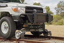
Many road–rail vehicles feature independent axles and suspension systems on each rail wheel. When this is combined with the presence of road wheels on the rail it becomes difficult to use the formulae above. Historically, road–rail vehicles have their front wheels set slightly toe-in, which has been found to minimise hunting whilst the vehicle is being driven on-rail.
See also[]
- Frictional contact mechanics
- Rail adhesion
- Rail profile
- Speed wobble
- Vehicle dynamics
- Wheelset
For general methods dealing with this class of problem, see
References[]
- ^ a b c Oxford English Dictionary (2nd ed.). Oxford University Press. 1989.
f. The action of a machine, instrument, system, etc., that is hunting (see hunt v. 7b); an undesirable oscillation about an equilibrium speed, position, or state.
- ^ https://www.talgo.com/en/rolling-stock/very-high-speed/350/
- ^ Tracking error will be zero if the path of the wheels runs absolutely straight along the track and the wheel pair is centered on the track.
- ^ See Curvature#Graph of a function for mathematical details. The approximate equality becomes equality only when the tracking error, y, has zero slope with respect to x. Since the tracking error will turn out to be a sine wave, the points of zero slope are at the points of maximum tracking error y. But the equality is approximately correct provided the slope of y is low.
- ^ Note that is negative when y is positive and conversely. The other equation for R, does not hold when y goes negative, since the radius R is not allowed to be negative (per mathematical definition). But after radius R is eliminated by combining the two equations, the resulting equation becomes correct by checking the two cases: y negative and y positive.
- ^ Iwnicki, p.7 formula 2.1
- ^ Carter, F. W. (July 25, 1928). "On the Stability of Running of Locomotives". Proceedings of the Royal Society. A. 121 (788): 585–610. Bibcode:1928RSPSA.121..585C. doi:10.1098/rspa.1928.0220.
- ^ Knothe, K. (2008). "History of wheel/rail contact mechanics: from Redtenbacher to Kalker". Vehicle System Dynamics. 46 (1–2): 9–26. doi:10.1080/00423110701586469. S2CID 109580328.
- ^ Wickens, A. H. (1965–66). "The Dynamics of Railway Vehicles on Straight Track: Fundamental Considerations of Lateral Stability". Proceedings of the Institution of Mechanical Engineers: 29–.
- ^ Wickens, A. H.; Gilchrist, A. O.; Hobbs, A. E. W. (1969–70). "Suspension Design for High-Performance Two-Axle Freight Vehicles". Proceedings of the Institution of Mechanical Engineers: 22–.
- ^ Serajian, Reza (2013). "Parameters' changing influence with different lateral stiffnesses on nonlinear analysis of hunting behavior of a bogie". Journal of Measurements in Engineering: 195–206.
- ^ Serajian, Reza (2011). "Effects of the bogie and body inertia on the nonlinear wheel-set hunting recognized by the hopf bifurcation theory". Int J Auto Engng: 186–196.

- Iwnicki, Simon (2006). Handbook of railway vehicle dynamics. CRC Press.
- Shabana, Ahmed A.; et al. (2008). Railroad vehicle dynamics : a computational approach. CRC Press.
- Wickens, A H (Jan 1, 2003). Fundamentals of rail vehicle dynamics : guidance and lateral stability. Swets & Zeitlinger.
- Serajian, Reza (2013). Parameters' changing influence with different lateral stiffnesses on nonlinear analysis of hunting behavior of a bogie. CRC Press.
- Serajian, Reza (2011). Effects of the bogie and body inertia on the nonlinear wheel-set hunting recognized by the hopf bifurcation theory. CRC Press.
- Oscillation
- Rail technologies