Logistic regression

In statistics, the logistic model (or logit model) is used to model the probability of a certain class or event existing such as pass/fail, win/lose, alive/dead or healthy/sick. This can be extended to model several classes of events such as determining whether an image contains a cat, dog, lion, etc. Each object being detected in the image would be assigned a probability between 0 and 1, with a sum of one.

Logistic regression is a statistical model that in its basic form uses a logistic function to model a binary dependent variable, although many more complex extensions exist. In regression analysis, logistic regression^[1] (or logit regression) is estimating the parameters of a logistic model (a form of binary regression). Mathematically, a binary logistic model has a dependent variable with two possible values, such as pass/fail which is represented by an indicator variable, where the two values are labeled "0" and "1". In the logistic model, the log-odds (the logarithm of the odds) for the value labeled "1" is a linear combination of one or more independent variables ("predictors"); the independent variables can each be a binary variable (two classes, coded by an indicator variable) or a continuous variable (any real value). The corresponding probability of the value labeled "1" can vary between 0 (certainly the value "0") and 1 (certainly the value "1"), hence the labeling; the function that converts log-odds to probability is the logistic function, hence the name. The unit of measurement for the log-odds scale is called a logit, from logistic unit, hence the alternative names. Analogous models with a different sigmoid function instead of the logistic function can also be used, such as the probit model; the defining characteristic of the logistic model is that increasing one of the independent variables multiplicatively scales the odds of the given outcome at a constant rate, with each independent variable having its own parameter; for a binary dependent variable this generalizes the odds ratio.

In a binary logistic regression model, the dependent variable has two levels (categorical). Outputs with more than two values are modeled by multinomial logistic regression and, if the multiple categories are ordered, by ordinal logistic regression (for example the proportional odds ordinal logistic model^[2]). The logistic regression model itself simply models probability of output in terms of input and does not perform statistical classification (it is not a classifier), though it can be used to make a classifier, for instance by choosing a cutoff value and classifying inputs with probability greater than the cutoff as one class, below the cutoff as the other; this is a common way to make a binary classifier. The coefficients are generally not computed by a closed-form expression, unlike linear least squares; see § Model fitting. The logistic regression as a general statistical model was originally developed and popularized primarily by Joseph Berkson,^[3] beginning in Berkson (1944) harvtxt error: no target: CITEREFBerkson1944 (help), where he coined "logit"; see § History.

Part of a series on
Regression analysis
Models
Linear regression Simple regression Polynomial regression General linear model
Generalized linear model Discrete choice Binomial regression Binary regression Logistic regression Multinomial logistic regression Mixed logit Probit Multinomial probit Ordered logit Ordered probit Poisson
Multilevel model Fixed effects Random effects Linear mixed-effects model Nonlinear mixed-effects model
Nonlinear regression Nonparametric Semiparametric Robust Quantile Isotonic Principal components Least angle Local Segmented
Errors-in-variables
Estimation
Least squares Linear Non-linear
Ordinary Weighted Generalized
Partial Total Non-negative Ridge regression Regularized
Least absolute deviations Iteratively reweighted Bayesian Bayesian multivariate
Background
Regression validation Mean and predicted response Errors and residuals Goodness of fit Studentized residual Gauss–Markov theorem
Mathematics portal
v t

Applications[]

Logistic regression is used in various fields, including machine learning, most medical fields, and social sciences. For example, the Trauma and Injury Severity Score (TRISS), which is widely used to predict mortality in injured patients, was originally developed by Boyd et al. using logistic regression.^[4] Many other medical scales used to assess severity of a patient have been developed using logistic regression.^[5][6][7][8] Logistic regression may be used to predict the risk of developing a given disease (e.g. diabetes; coronary heart disease), based on observed characteristics of the patient (age, sex, body mass index, results of various blood tests, etc.).^[9][10] Another example might be to predict whether a Nepalese voter will vote Nepali Congress or Communist Party of Nepal or Any Other Party, based on age, income, sex, race, state of residence, votes in previous elections, etc.^[11] The technique can also be used in engineering, especially for predicting the probability of failure of a given process, system or product.^[12][13] It is also used in marketing applications such as prediction of a customer's propensity to purchase a product or halt a subscription, etc.^[14] In economics it can be used to predict the likelihood of a person ending up in the labor force, and a business application would be to predict the likelihood of a homeowner defaulting on a mortgage. Conditional random fields, an extension of logistic regression to sequential data, are used in natural language processing.

Examples[]

Logistic model[]

Let us try to understand logistic regression by considering a logistic model with given parameters, then seeing how the coefficients can be estimated from data. Consider a model with two predictors, ${\displaystyle x_{1}}$ and ${\displaystyle x_{2}}$, and one binary (Bernoulli) response variable ${\displaystyle Y}$, which we denote ${\displaystyle p=P(Y=1)}$. We assume a linear relationship between the predictor variables and the log-odds (also called logit) of the event that ${\displaystyle Y=1}$. This linear relationship can be written in the following mathematical form (where ℓ is the log-odds, ${\displaystyle b}$ is the base of the logarithm, and ${\displaystyle \beta _{i}}$ are parameters of the model):

${\displaystyle \ell =\log _{b}{\frac {p}{1-p}}=\beta _{0}+\beta _{1}x_{1}+\beta _{2}x_{2}}$

We can recover the odds by exponentiating the log-odds:

${\displaystyle {\frac {p}{1-p}}=b^{\beta _{0}+\beta _{1}x_{1}+\beta _{2}x_{2}}}$.

By simple algebraic manipulation (and dividing numerator and denominator by ${\displaystyle b^{\beta _{0}+\beta _{1}x_{1}+\beta _{2}x_{2}}}$), the probability that ${\displaystyle Y=1}$ is

${\displaystyle p={\frac {b^{\beta _{0}+\beta _{1}x_{1}+\beta _{2}x_{2}}}{b^{\beta _{0}+\beta _{1}x_{1}+\beta _{2}x_{2}}+1}}={\frac {1}{1+b^{-(\beta _{0}+\beta _{1}x_{1}+\beta _{2}x_{2})}}}=S_{b}(\beta _{0}+\beta _{1}x_{1}+\beta _{2}x_{2})}$.

Where ${\displaystyle S_{b}}$ is the sigmoid function with base ${\displaystyle b}$. The above formula shows that once ${\displaystyle \beta _{i}}$ are fixed, we can easily compute either the log-odds that ${\displaystyle Y=1}$ for a given observation, or the probability that ${\displaystyle Y=1}$ for a given observation. The main use-case of a logistic model is to be given an observation ${\displaystyle (x_{1},x_{2})}$, and estimate the probability ${\displaystyle p}$ that ${\displaystyle Y=1}$. In most applications, the base ${\displaystyle b}$ of the logarithm is usually taken to be e. However, in some cases it can be easier to communicate results by working in base 2, or base 10.

We consider an example with ${\displaystyle b=10}$, and coefficients ${\displaystyle \beta _{0}=-3}$, ${\displaystyle \beta _{1}=1}$, and ${\displaystyle \beta _{2}=2}$. To be concrete, the model is

${\displaystyle \log _{10}{\frac {p}{1-p}}=\ell =-3+x_{1}+2x_{2}}$

where ${\displaystyle p}$ is the probability of the event that ${\displaystyle Y=1}$.

This can be interpreted as follows:

• ${\displaystyle \beta _{0}=-3}$ is the y-intercept. It is the log-odds of the event that ${\displaystyle Y=1}$, when the predictors ${\displaystyle x_{1}=x_{2}=0}$. By exponentiating, we can see that when ${\displaystyle x_{1}=x_{2}=0}$ the odds of the event that ${\displaystyle Y=1}$ are 1-to-1000, or ${\displaystyle 10^{-3}}$. Similarly, the probability of the event that ${\displaystyle Y=1}$ when ${\displaystyle x_{1}=x_{2}=0}$ can be computed as ${\displaystyle 1/(1000+1)=1/1001}$.
• ${\displaystyle \beta _{1}=1}$ means that increasing ${\displaystyle x_{1}}$ by 1 increases the log-odds by ${\displaystyle 1}$. So if ${\displaystyle x_{1}}$ increases by 1, the odds that ${\displaystyle Y=1}$ increase by a factor of ${\displaystyle 10^{1}}$. Note that the probability of ${\displaystyle Y=1}$ has also increased, but it has not increased by as much as the odds have increased.
• ${\displaystyle \beta _{2}=2}$ means that increasing ${\displaystyle x_{2}}$ by 1 increases the log-odds by ${\displaystyle 2}$. So if ${\displaystyle x_{2}}$ increases by 1, the odds that ${\displaystyle Y=1}$ increase by a factor of ${\displaystyle 10^{2}.}$ Note how the effect of ${\displaystyle x_{2}}$ on the log-odds is twice as great as the effect of ${\displaystyle x_{1}}$, but the effect on the odds is 10 times greater. But the effect on the probability of ${\displaystyle Y=1}$ is not as much as 10 times greater, it's only the effect on the odds that is 10 times greater.

In order to estimate the parameters ${\displaystyle \beta _{i}}$ from data, one must do logistic regression.

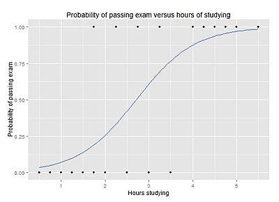
Probability of passing an exam versus hours of study[]

To answer the following question:

A group of 20 students spends between 0 and 6 hours studying for an exam. How does the number of hours spent studying affect the probability of the student passing the exam?

The reason for using logistic regression for this problem is that the values of the dependent variable, pass and fail, while represented by "1" and "0", are not cardinal numbers. If the problem was changed so that pass/fail was replaced with the grade 0–100 (cardinal numbers), then simple regression analysis could be used.

The table shows the number of hours each student spent studying, and whether they passed (1) or failed (0).

Hours	0.50	0.75	1.00	1.25	1.50	1.75	1.75	2.00	2.25	2.50	2.75	3.00	3.25	3.50	4.00	4.25	4.50	4.75	5.00	5.50
Pass	0	0	0	0	0	0	1	0	1	0	1	0	1	0	1	1	1	1	1	1

The graph shows the probability of passing the exam versus the number of hours studying, with the logistic regression curve fitted to the data.

The logistic regression analysis gives the following output.

	Coefficient	Std.Error	z-value	P-value (Wald)
Intercept	−4.0777	1.7610	−2.316	0.0206
Hours	1.5046	0.6287	2.393	0.0167

The output indicates that hours studying is significantly associated with the probability of passing the exam (${\displaystyle p=0.0167}$, Wald test). The output also provides the coefficients for ${\displaystyle {\text{Intercept}}=-4.0777}$ and ${\displaystyle {\text{Hours}}=1.5046}$. These coefficients are entered in the logistic regression equation to estimate the odds (probability) of passing the exam:

${\displaystyle {\begin{aligned}{\text{Log-odds of passing exam}}&=1.5046\cdot {\text{Hours}}-4.0777=1.5046\cdot ({\text{Hours}}-2.71)\\{\text{Odds of passing exam}}&=\exp \left(1.5046\cdot {\text{Hours}}-4.0777\right)=\exp \left(1.5046\cdot ({\text{Hours}}-2.71)\right)\\{\text{Probability of passing exam}}&={\frac {1}{1+\exp \left(-\left(1.5046\cdot {\text{Hours}}-4.0777\right)\right)}}\end{aligned}}}$

One additional hour of study is estimated to increase log-odds of passing by 1.5046, so multiplying odds of passing by ${\displaystyle \exp(1.5046)\approx 4.5.}$ The form with the x-intercept (2.71) shows that this estimates even odds (log-odds 0, odds 1, probability 1/2) for a student who studies 2.71 hours.

For example, for a student who studies 2 hours, entering the value ${\displaystyle {\text{Hours}}=2}$ in the equation gives the estimated probability of passing the exam of 0.26:

${\displaystyle {\text{Probability of passing exam}}={\frac {1}{1+\exp \left(-\left(1.5046\cdot 2-4.0777\right)\right)}}=0.26}$

Similarly, for a student who studies 4 hours, the estimated probability of passing the exam is 0.87:

${\displaystyle {\text{Probability of passing exam}}={\frac {1}{1+\exp \left(-\left(1.5046\cdot 4-4.0777\right)\right)}}=0.87}$

This table shows the probability of passing the exam for several values of hours studying.

Hours of study	Passing exam
	Log-odds	Odds	Probability
1	−2.57	0.076 ≈ 1:13.1	0.07
2	−1.07	0.34 ≈ 1:2.91	0.26
3	0.44	1.55	0.61
4	1.94	6.96	0.87
5	3.45	31.4	0.97

The output from the logistic regression analysis gives a p-value of ${\displaystyle p=0.0167}$, which is based on the Wald z-score. Rather than the Wald method, the recommended method^{[citation needed]} to calculate the p-value for logistic regression is the likelihood-ratio test (LRT), which for this data gives ${\displaystyle p=0.0006}$.

Discussion[]

Logistic regression can be binomial, ordinal or multinomial. Binomial or binary logistic regression deals with situations in which the observed outcome for a dependent variable can have only two possible types, "0" and "1" (which may represent, for example, "dead" vs. "alive" or "win" vs. "loss"). Multinomial logistic regression deals with situations where the outcome can have three or more possible types (e.g., "disease A" vs. "disease B" vs. "disease C") that are not ordered. Ordinal logistic regression deals with dependent variables that are ordered.

In binary logistic regression, the outcome is usually coded as "0" or "1", as this leads to the most straightforward interpretation.^[15] If a particular observed outcome for the dependent variable is the noteworthy possible outcome (referred to as a "success" or an "instance" or a "case") it is usually coded as "1" and the contrary outcome (referred to as a "failure" or a "noninstance" or a "noncase") as "0". Binary logistic regression is used to predict the odds of being a case based on the values of the independent variables (predictors). The odds are defined as the probability that a particular outcome is a case divided by the probability that it is a noninstance.

Like other forms of regression analysis, logistic regression makes use of one or more predictor variables that may be either continuous or categorical. Unlike ordinary linear regression, however, logistic regression is used for predicting dependent variables that take membership in one of a limited number of categories (treating the dependent variable in the binomial case as the outcome of a Bernoulli trial) rather than a continuous outcome. Given this difference, the assumptions of linear regression are violated. In particular, the residuals cannot be normally distributed. In addition, linear regression may make nonsensical predictions for a binary dependent variable. What is needed is a way to convert a binary variable into a continuous one that can take on any real value (negative or positive). To do that, binomial logistic regression first calculates the odds of the event happening for different levels of each independent variable, and then takes its logarithm to create a continuous criterion as a transformed version of the dependent variable. The logarithm of the odds is the logit of the probability, the logit is defined as follows:

${\displaystyle \operatorname {logit} p=\ln {\frac {p}{1-p}}\quad {\text{for }}0<p<1\,.}$

Although the dependent variable in logistic regression is Bernoulli, the logit is on an unrestricted scale.^[15] The logit function is the link function in this kind of generalized linear model, i.e.

${\displaystyle \operatorname {logit} \operatorname {\mathcal {E}} (Y)=\beta _{0}+\beta _{1}x}$

Y is the Bernoulli-distributed response variable and x is the predictor variable; the β values are the linear parameters.

The logit of the probability of success is then fitted to the predictors. The predicted value of the logit is converted back into predicted odds, via the inverse of the natural logarithm – the exponential function. Thus, although the observed dependent variable in binary logistic regression is a 0-or-1 variable, the logistic regression estimates the odds, as a continuous variable, that the dependent variable is a ‘success’. In some applications, the odds are all that is needed. In others, a specific yes-or-no prediction is needed for whether the dependent variable is or is not a ‘success’; this categorical prediction can be based on the computed odds of success, with predicted odds above some chosen cutoff value being translated into a prediction of success.

The assumption of linear predictor effects can easily be relaxed using techniques such as spline functions.^[16]

Logistic regression vs. other approaches[]

Logistic regression measures the relationship between the categorical dependent variable and one or more independent variables by estimating probabilities using a logistic function, which is the cumulative distribution function of logistic distribution. Thus, it treats the same set of problems as probit regression using similar techniques, with the latter using a cumulative normal distribution curve instead. Equivalently, in the latent variable interpretations of these two methods, the first assumes a standard logistic distribution of errors and the second a standard normal distribution of errors.^[17]

Logistic regression can be seen as a special case of the generalized linear model and thus analogous to linear regression. The model of logistic regression, however, is based on quite different assumptions (about the relationship between the dependent and independent variables) from those of linear regression. In particular, the key differences between these two models can be seen in the following two features of logistic regression. First, the conditional distribution ${\displaystyle y\mid x}$ is a Bernoulli distribution rather than a Gaussian distribution, because the dependent variable is binary. Second, the predicted values are probabilities and are therefore restricted to (0,1) through the logistic distribution function because logistic regression predicts the probability of particular outcomes rather than the outcomes themselves.

Logistic regression is an alternative to Fisher's 1936 method, linear discriminant analysis.^[18] If the assumptions of linear discriminant analysis hold, the conditioning can be reversed to produce logistic regression. The converse is not true, however, because logistic regression does not require the multivariate normal assumption of discriminant analysis.^[19]

Latent variable interpretation[]

The logistic regression can be understood simply as finding the ${\displaystyle \beta }$ parameters that best fit:

${\displaystyle y={\begin{cases}1&\beta _{0}+\beta _{1}x+\varepsilon >0\\0&{\text{else}}\end{cases}}}$

where ${\displaystyle \varepsilon }$ is an error distributed by the standard logistic distribution. (If the standard normal distribution is used instead, it is a probit model.)

The associated latent variable is ${\displaystyle y'=\beta _{0}+\beta _{1}x+\varepsilon }$. The error term ${\displaystyle \varepsilon }$ is not observed, and so the ${\displaystyle y'}$ is also an unobservable, hence termed "latent" (the observed data are values of ${\displaystyle y}$ and ${\displaystyle x}$). Unlike ordinary regression, however, the ${\displaystyle \beta }$ parameters cannot be expressed by any direct formula of the ${\displaystyle y}$ and ${\displaystyle x}$ values in the observed data. Instead they are to be found by an iterative search process, usually implemented by a software program, that finds the maximum of a complicated "likelihood expression" that is a function of all of the observed ${\displaystyle y}$ and ${\displaystyle x}$ values. The estimation approach is explained below.

Logistic function, odds, odds ratio, and logit[]

Definition of the logistic function[]

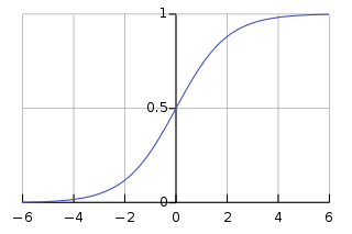
An explanation of logistic regression can begin with an explanation of the standard logistic function. The logistic function is a sigmoid function, which takes any real input ${\displaystyle t}$, and outputs a value between zero and one.^[15] For the logit, this is interpreted as taking input log-odds and having output probability. The standard logistic function ${\displaystyle \sigma :\mathbb {R} \rightarrow (0,1)}$ is defined as follows:

${\displaystyle \sigma (t)={\frac {e^{t}}{e^{t}+1}}={\frac {1}{1+e^{-t}}}}$

A graph of the logistic function on the t-interval (−6,6) is shown in Figure 1.

Let us assume that ${\displaystyle t}$ is a linear function of a single explanatory variable ${\displaystyle x}$ (the case where ${\displaystyle t}$ is a linear combination of multiple explanatory variables is treated similarly). We can then express ${\displaystyle t}$ as follows:

${\displaystyle t=\beta _{0}+\beta _{1}x}$

And the general logistic function ${\displaystyle p:\mathbb {R} \rightarrow (0,1)}$ can now be written as:

${\displaystyle p(x)=\sigma (t)={\frac {1}{1+e^{-(\beta _{0}+\beta _{1}x)}}}}$

In the logistic model, ${\displaystyle p(x)}$ is interpreted as the probability of the dependent variable ${\displaystyle Y}$ equaling a success/case rather than a failure/non-case. It's clear that the response variables ${\displaystyle Y_{i}}$ are not identically distributed: ${\displaystyle P(Y_{i}=1\mid X)}$ differs from one data point ${\displaystyle X_{i}}$ to another, though they are independent given design matrix ${\displaystyle X}$ and shared parameters ${\displaystyle \beta }$.^[9]

Definition of the inverse of the logistic function[]

We can now define the logit (log odds) function as the inverse ${\displaystyle g=\sigma ^{-1}}$ of the standard logistic function. It is easy to see that it satisfies:

${\displaystyle g(p(x))=\sigma ^{-1}(p(x))=\operatorname {logit} p(x)=\ln \left({\frac {p(x)}{1-p(x)}}\right)=\beta _{0}+\beta _{1}x,}$

and equivalently, after exponentiating both sides we have the odds:

${\displaystyle {\frac {p(x)}{1-p(x)}}=e^{\beta _{0}+\beta _{1}x}.}$

Interpretation of these terms[]

In the above equations, the terms are as follows:

• ${\displaystyle g}$ is the logit function. The equation for ${\displaystyle g(p(x))}$ illustrates that the logit (i.e., log-odds or natural logarithm of the odds) is equivalent to the linear regression expression.
• ${\displaystyle \ln }$ denotes the natural logarithm.
• ${\displaystyle p(x)}$ is the probability that the dependent variable equals a case, given some linear combination of the predictors. The formula for ${\displaystyle p(x)}$ illustrates that the probability of the dependent variable equaling a case is equal to the value of the logistic function of the linear regression expression. This is important in that it shows that the value of the linear regression expression can vary from negative to positive infinity and yet, after transformation, the resulting expression for the probability ${\displaystyle p(x)}$ ranges between 0 and 1.
• ${\displaystyle \beta _{0}}$ is the intercept from the linear regression equation (the value of the criterion when the predictor is equal to zero).
• ${\displaystyle \beta _{1}x}$ is the regression coefficient multiplied by some value of the predictor.
• base ${\displaystyle e}$ denotes the exponential function.

Definition of the odds[]

The odds of the dependent variable equaling a case (given some linear combination ${\displaystyle x}$ of the predictors) is equivalent to the exponential function of the linear regression expression. This illustrates how the logit serves as a link function between the probability and the linear regression expression. Given that the logit ranges between negative and positive infinity, it provides an adequate criterion upon which to conduct linear regression and the logit is easily converted back into the odds.^[15]

So we define odds of the dependent variable equaling a case (given some linear combination ${\displaystyle x}$ of the predictors) as follows:

${\displaystyle {\text{odds}}=e^{\beta _{0}+\beta _{1}x}.}$

The odds ratio[]

For a continuous independent variable the odds ratio can be defined as:

${\displaystyle \mathrm {OR} ={\frac {\operatorname {odds} (x+1)}{\operatorname {odds} (x)}}={\frac {\left({\frac {F(x+1)}{1-F(x+1)}}\right)}{\left({\frac {F(x)}{1-F(x)}}\right)}}={\frac {e^{\beta _{0}+\beta _{1}(x+1)}}{e^{\beta _{0}+\beta _{1}x}}}=e^{\beta _{1}}}$

This exponential relationship provides an interpretation for ${\displaystyle \beta _{1}}$: The odds multiply by ${\displaystyle e^{\beta _{1}}}$ for every 1-unit increase in x.^[20]

For a binary independent variable the odds ratio is defined as ${\displaystyle {\frac {ad}{bc}}}$ where a, b, c and d are cells in a 2×2 contingency table.^[21]

Multiple explanatory variables[]

If there are multiple explanatory variables, the above expression ${\displaystyle \beta _{0}+\beta _{1}x}$ can be revised to ${\displaystyle \beta _{0}+\beta _{1}x_{1}+\beta _{2}x_{2}+\cdots +\beta _{m}x_{m}=\beta _{0}+\sum _{i=1}^{m}\beta _{i}x_{i}}$. Then when this is used in the equation relating the log odds of a success to the values of the predictors, the linear regression will be a multiple regression with m explanators; the parameters ${\displaystyle \beta _{j}}$ for all j = 0, 1, 2, ..., m are all estimated.

Again, the more traditional equations are:

${\displaystyle \log {\frac {p}{1-p}}=\beta _{0}+\beta _{1}x_{1}+\beta _{2}x_{2}+\cdots +\beta _{m}x_{m}}$

and

${\displaystyle p={\frac {1}{1+b^{-(\beta _{0}+\beta _{1}x_{1}+\beta _{2}x_{2}+\cdots +\beta _{m}x_{m})}}}}$

where usually ${\displaystyle b=e}$.

Model fitting[]

This section needs expansion. You can help by . (October 2016)

Logistic regression is an important machine learning algorithm. The goal is to model the probability of a random variable ${\displaystyle Y}$ being 0 or 1 given experimental data.^[22]

Consider a generalized linear model function parameterized by ${\displaystyle \theta }$,

${\displaystyle h_{\theta }(X)={\frac {1}{1+e^{-\theta ^{T}X}}}=\Pr(Y=1\mid X;\theta )}$

Therefore,

${\displaystyle \Pr(Y=0\mid X;\theta )=1-h_{\theta }(X)}$

and since ${\displaystyle Y\in \{0,1\}}$, we see that ${\displaystyle \Pr(y\mid X;\theta )}$ is given by ${\displaystyle \Pr(y\mid X;\theta )=h_{\theta }(X)^{y}(1-h_{\theta }(X))^{(1-y)}.}$ We now calculate the likelihood function assuming that all the observations in the sample are independently Bernoulli distributed,

${\displaystyle {\begin{aligned}L(\theta \mid y;x)&=\Pr(Y\mid X;\theta )\\&=\prod _{i}\Pr(y_{i}\mid x_{i};\theta )\\&=\prod _{i}h_{\theta }(x_{i})^{y_{i}}(1-h_{\theta }(x_{i}))^{(1-y_{i})}\end{aligned}}}$

Typically, the log likelihood is maximized,

${\displaystyle N^{-1}\log L(\theta \mid y;x)=N^{-1}\sum _{i=1}^{N}\log \Pr(y_{i}\mid x_{i};\theta )}$

which is maximized using optimization techniques such as gradient descent.

Assuming the ${\displaystyle (x,y)}$ pairs are drawn uniformly from the underlying distribution, then in the limit of large N,

${\displaystyle {\begin{aligned}&\lim \limits _{N\rightarrow +\infty }N^{-1}\sum _{i=1}^{N}\log \Pr(y_{i}\mid x_{i};\theta )=\sum _{x\in {\mathcal {X}}}\sum _{y\in {\mathcal {Y}}}\Pr(X=x,Y=y)\log \Pr(Y=y\mid X=x;\theta )\\[6pt]={}&\sum _{x\in {\mathcal {X}}}\sum _{y\in {\mathcal {Y}}}\Pr(X=x,Y=y)\left(-\log {\frac {\Pr(Y=y\mid X=x)}{\Pr(Y=y\mid X=x;\theta )}}+\log \Pr(Y=y\mid X=x)\right)\\[6pt]={}&-D_{\text{KL}}(Y\parallel Y_{\theta })-H(Y\mid X)\end{aligned}}}$

where ${\displaystyle H(Y\mid X)}$ is the conditional entropy and ${\displaystyle D_{\text{KL}}}$ is the Kullback–Leibler divergence. This leads to the intuition that by maximizing the log-likelihood of a model, you are minimizing the KL divergence of your model from the maximal entropy distribution. Intuitively searching for the model that makes the fewest assumptions in its parameters.

"Rule of ten"[]

A widely used rule of thumb, the "one in ten rule", states that logistic regression models give stable values for the explanatory variables if based on a minimum of about 10 events per explanatory variable (EPV); where event denotes the cases belonging to the less frequent category in the dependent variable. Thus a study designed to use ${\displaystyle k}$ explanatory variables for an event (e.g. myocardial infarction) expected to occur in a proportion ${\displaystyle p}$ of participants in the study will require a total of ${\displaystyle 10k/p}$ participants. However, there is considerable debate about the reliability of this rule, which is based on simulation studies and lacks a secure theoretical underpinning.^[23] According to some authors^[24] the rule is overly conservative, some circumstances; with the authors stating "If we (somewhat subjectively) regard confidence interval coverage less than 93 percent, type I error greater than 7 percent, or relative bias greater than 15 percent as problematic, our results indicate that problems are fairly frequent with 2–4 EPV, uncommon with 5–9 EPV, and still observed with 10–16 EPV. The worst instances of each problem were not severe with 5–9 EPV and usually comparable to those with 10–16 EPV".^[25]

Others have found results that are not consistent with the above, using different criteria. A useful criterion is whether the fitted model will be expected to achieve the same predictive discrimination in a new sample as it appeared to achieve in the model development sample. For that criterion, 20 events per candidate variable may be required.^[26] Also, one can argue that 96 observations are needed only to estimate the model's intercept precisely enough that the margin of error in predicted probabilities is ±0.1 with an 0.95 confidence level.^[16]

Maximum likelihood estimation (MLE)[]

The regression coefficients are usually estimated using maximum likelihood estimation.^[27][28] Unlike linear regression with normally distributed residuals, it is not possible to find a closed-form expression for the coefficient values that maximize the likelihood function, so that an iterative process must be used instead; for example Newton's method. This process begins with a tentative solution, revises it slightly to see if it can be improved, and repeats this revision until no more improvement is made, at which point the process is said to have converged.^[27]

In some instances, the model may not reach convergence. Non-convergence of a model indicates that the coefficients are not meaningful because the iterative process was unable to find appropriate solutions. A failure to converge may occur for a number of reasons: having a large ratio of predictors to cases, multicollinearity, sparseness, or complete separation.

• Having a large ratio of variables to cases results in an overly conservative Wald statistic (discussed below) and can lead to non-convergence. Regularized logistic regression is specifically intended to be used in this situation.
• Multicollinearity refers to unacceptably high correlations between predictors. As multicollinearity increases, coefficients remain unbiased but standard errors increase and the likelihood of model convergence decreases.^[27] To detect multicollinearity amongst the predictors, one can conduct a linear regression analysis with the predictors of interest for the sole purpose of examining the tolerance statistic ^[27] used to assess whether multicollinearity is unacceptably high.
• Sparseness in the data refers to having a large proportion of empty cells (cells with zero counts). Zero cell counts are particularly problematic with categorical predictors. With continuous predictors, the model can infer values for the zero cell counts, but this is not the case with categorical predictors. The model will not converge with zero cell counts for categorical predictors because the natural logarithm of zero is an undefined value so that the final solution to the model cannot be reached. To remedy this problem, researchers may collapse categories in a theoretically meaningful way or add a constant to all cells.^[27]
• Another numerical problem that may lead to a lack of convergence is complete separation, which refers to the instance in which the predictors perfectly predict the criterion – all cases are accurately classified. In such instances, one should reexamine the data, as there is likely some kind of error.^{[15][further explanation needed]}
• One can also take semi-parametric or non-parametric approaches, e.g., via local-likelihood or nonparametric quasi-likelihood methods, which avoid assumptions of a parametric form for the index function and is robust to the choice of the link function (e.g., probit or logit).^[29]

Cross-entropy Loss function[]

In machine learning applications where logistic regression is used for binary classification, the MLE minimises the Cross entropy loss function.

Iteratively reweighted least squares (IRLS)[]

Binary logistic regression (${\displaystyle y=0}$ or ${\displaystyle y=1}$) can, for example, be calculated using iteratively reweighted least squares (IRLS), which is equivalent to maximizing the log-likelihood of a Bernoulli distributed process using Newton's method. If the problem is written in vector matrix form, with parameters ${\displaystyle \mathbf {w} ^{T}=[\beta _{0},\beta _{1},\beta _{2},\ldots ]}$, explanatory variables ${\displaystyle \mathbf {x} (i)=[1,x_{1}(i),x_{2}(i),\ldots ]^{T}}$ and expected value of the Bernoulli distribution ${\displaystyle \mu (i)={\frac {1}{1+e^{-\mathbf {w} ^{T}\mathbf {x} (i)}}}}$, the parameters ${\displaystyle \mathbf {w} }$ can be found using the following iterative algorithm:

${\displaystyle \mathbf {w} _{k+1}=\left(\mathbf {X} ^{T}\mathbf {S} _{k}\mathbf {X} \right)^{-1}\mathbf {X} ^{T}\left(\mathbf {S} _{k}\mathbf {X} \mathbf {w} _{k}+\mathbf {y} -\mathbf {\boldsymbol {\mu }} _{k}\right)}$

where ${\displaystyle \mathbf {S} =\operatorname {diag} (\mu (i)(1-\mu (i)))}$ is a diagonal weighting matrix, ${\displaystyle {\boldsymbol {\mu }}=[\mu (1),\mu (2),\ldots ]}$ the vector of expected values,

${\displaystyle \mathbf {X} ={\begin{bmatrix}1&x_{1}(1)&x_{2}(1)&\ldots \\1&x_{1}(2)&x_{2}(2)&\ldots \\\vdots &\vdots &\vdots \end{bmatrix}}}$

The regressor matrix and ${\displaystyle \mathbf {y} (i)=[y(1),y(2),\ldots ]^{T}}$ the vector of response variables. More details can be found in the literature.^[30]

Evaluating goodness of fit[]

Goodness of fit in linear regression models is generally measured using R². Since this has no direct analog in logistic regression, various methods^[31]:ch.21 including the following can be used instead.

Deviance and likelihood ratio tests[]

In linear regression analysis, one is concerned with partitioning variance via the sum of squares calculations – variance in the criterion is essentially divided into variance accounted for by the predictors and residual variance. In logistic regression analysis, deviance is used in lieu of a sum of squares calculations.^[32] Deviance is analogous to the sum of squares calculations in linear regression^[15] and is a measure of the lack of fit to the data in a logistic regression model.^[32] When a "saturated" model is available (a model with a theoretically perfect fit), deviance is calculated by comparing a given model with the saturated model.^[15] This computation gives the likelihood-ratio test:^[15]

${\displaystyle D=-2\ln {\frac {\text{likelihood of the fitted model}}{\text{likelihood of the saturated model}}}.}$

In the above equation, D represents the deviance and ln represents the natural logarithm. The log of this likelihood ratio (the ratio of the fitted model to the saturated model) will produce a negative value, hence the need for a negative sign. D can be shown to follow an approximate chi-squared distribution.^[15] Smaller values indicate better fit as the fitted model deviates less from the saturated model. When assessed upon a chi-square distribution, nonsignificant chi-square values indicate very little unexplained variance and thus, good model fit. Conversely, a significant chi-square value indicates that a significant amount of the variance is unexplained.

When the saturated model is not available (a common case), deviance is calculated simply as −2·(log likelihood of the fitted model), and the reference to the saturated model's log likelihood can be removed from all that follows without harm.

Two measures of deviance are particularly important in logistic regression: null deviance and model deviance. The null deviance represents the difference between a model with only the intercept (which means "no predictors") and the saturated model. The model deviance represents the difference between a model with at least one predictor and the saturated model.^[32] In this respect, the null model provides a baseline upon which to compare predictor models. Given that deviance is a measure of the difference between a given model and the saturated model, smaller values indicate better fit. Thus, to assess the contribution of a predictor or set of predictors, one can subtract the model deviance from the null deviance and assess the difference on a ${\displaystyle \chi _{s-p}^{2},}$ chi-square distribution with degrees of freedom^[15] equal to the difference in the number of parameters estimated.

Let

${\displaystyle {\begin{aligned}D_{\text{null}}&=-2\ln {\frac {\text{likelihood of null model}}{\text{likelihood of the saturated model}}}\\[6pt]D_{\text{fitted}}&=-2\ln {\frac {\text{likelihood of fitted model}}{\text{likelihood of the saturated model}}}.\end{aligned}}}$

Then the difference of both is:

${\displaystyle {\begin{aligned}D_{\text{null}}-D_{\text{fitted}}&=-2\left(\ln {\frac {\text{likelihood of null model}}{\text{likelihood of the saturated model}}}-\ln {\frac {\text{likelihood of fitted model}}{\text{likelihood of the saturated model}}}\right)\\[6pt]&=-2\ln {\frac {\left({\dfrac {\text{likelihood of null model}}{\text{likelihood of the saturated model}}}\right)}{\left({\dfrac {\text{likelihood of fitted model}}{\text{likelihood of the saturated model}}}\right)}}\\[6pt]&=-2\ln {\frac {\text{likelihood of the null model}}{\text{likelihood of fitted model}}}.\end{aligned}}}$

If the model deviance is significantly smaller than the null deviance then one can conclude that the predictor or set of predictors significantly improved model fit. This is analogous to the F-test used in linear regression analysis to assess the significance of prediction.^[32]

Pseudo-R-squared[]

In linear regression the squared multiple correlation, R² is used to assess goodness of fit as it represents the proportion of variance in the criterion that is explained by the predictors.^[32] In logistic regression analysis, there is no agreed upon analogous measure, but there are several competing measures each with limitations.^[32][33]

Four of the most commonly used indices and one less commonly used one are examined on this page:

• Likelihood ratio R²_L
• Cox and Snell R²_CS
• Nagelkerke R²_N
• McFadden R²_McF
• Tjur R²_T

R²_L is given by Cohen:^[32]

${\displaystyle R_{\text{L}}^{2}={\frac {D_{\text{null}}-D_{\text{fitted}}}{D_{\text{null}}}}.}$

This is the most analogous index to the squared multiple correlations in linear regression.^[27] It represents the proportional reduction in the deviance wherein the deviance is treated as a measure of variation analogous but not identical to the variance in linear regression analysis.^[27] One limitation of the likelihood ratio R² is that it is not monotonically related to the odds ratio,^[32] meaning that it does not necessarily increase as the odds ratio increases and does not necessarily decrease as the odds ratio decreases.

R²_CS is an alternative index of goodness of fit related to the R² value from linear regression.^[33] It is given by:

${\displaystyle {\begin{aligned}R_{\text{CS}}^{2}&=1-\left({\frac {L_{0}}{L_{M}}}\right)^{2/n}\\[5pt]&=1-e^{2(\ln(L_{0})-\ln(L_{M}))/n}\end{aligned}}}$

where L_M and L₀ are the likelihoods for the model being fitted and the null model, respectively. The Cox and Snell index is problematic as its maximum value is ${\displaystyle 1-L_{0}^{2/n}}$. The highest this upper bound can be is 0.75, but it can easily be as low as 0.48 when the marginal proportion of cases is small.^[33]

R²_N provides a correction to the Cox and Snell R² so that the maximum value is equal to 1. Nevertheless, the Cox and Snell and likelihood ratio R²s show greater agreement with each other than either does with the Nagelkerke R².^[32] Of course, this might not be the case for values exceeding 0.75 as the Cox and Snell index is capped at this value. The likelihood ratio R² is often preferred to the alternatives as it is most analogous to R² in linear regression, is independent of the base rate (both Cox and Snell and Nagelkerke R²s increase as the proportion of cases increase from 0 to 0.5) and varies between 0 and 1.

R²_McF is defined as

${\displaystyle R_{\text{McF}}^{2}=1-{\frac {\ln(L_{M})}{\ln(L_{0})}},}$

and is preferred over R²_CS by Allison.^[33] The two expressions R²_McF and R²_CS are then related respectively by,

${\displaystyle {\begin{matrix}R_{\text{CS}}^{2}=1-\left({\dfrac {1}{L_{0}}}\right)^{\frac {2(R_{\text{McF}}^{2})}{n}}\\[1.5em]R_{\text{McF}}^{2}=-{\dfrac {n}{2}}\cdot {\dfrac {\ln(1-R_{\text{CS}}^{2})}{\ln L_{0}}}\end{matrix}}}$

However, Allison now prefers R²_T which is a relatively new measure developed by Tjur.^[34] It can be calculated in two steps:^[33]

1. For each level of the dependent variable, find the mean of the predicted probabilities of an event.
2. Take the absolute value of the difference between these means

A word of caution is in order when interpreting pseudo-R² statistics. The reason these indices of fit are referred to as pseudo R² is that they do not represent the proportionate reduction in error as the R² in linear regression does.^[32] Linear regression assumes homoscedasticity, that the error variance is the same for all values of the criterion. Logistic regression will always be heteroscedastic – the error variances differ for each value of the predicted score. For each value of the predicted score there would be a different value of the proportionate reduction in error. Therefore, it is inappropriate to think of R² as a proportionate reduction in error in a universal sense in logistic regression.^[32]

Hosmer–Lemeshow test[]

The Hosmer–Lemeshow test uses a test statistic that asymptotically follows a ${\displaystyle \chi ^{2}}$ distribution to assess whether or not the observed event rates match expected event rates in subgroups of the model population. This test is considered to be obsolete by some statisticians because of its dependence on arbitrary binning of predicted probabilities and relative low power.^[35]

Coefficients[]

After fitting the model, it is likely that researchers will want to examine the contribution of individual predictors. To do so, they will want to examine the regression coefficients. In linear regression, the regression coefficients represent the change in the criterion for each unit change in the predictor.^[32] In logistic regression, however, the regression coefficients represent the change in the logit for each unit change in the predictor. Given that the logit is not intuitive, researchers are likely to focus on a predictor's effect on the exponential function of the regression coefficient – the odds ratio (see definition). In linear regression, the significance of a regression coefficient is assessed by computing a t test. In logistic regression, there are several different tests designed to assess the significance of an individual predictor, most notably the likelihood ratio test and the Wald statistic.

Likelihood ratio test[]

The likelihood-ratio test discussed above to assess model fit is also the recommended procedure to assess the contribution of individual "predictors" to a given model.^[15][27][32] In the case of a single predictor model, one simply compares the deviance of the predictor model with that of the null model on a chi-square distribution with a single degree of freedom. If the predictor model has significantly smaller deviance (c.f chi-square using the difference in degrees of freedom of the two models), then one can conclude that there is a significant association between the "predictor" and the outcome. Although some common statistical packages (e.g. SPSS) do provide likelihood ratio test statistics, without this computationally intensive test it would be more difficult to assess the contribution of individual predictors in the multiple logistic regression case.^{[citation needed]} To assess the contribution of individual predictors one can enter the predictors hierarchically, comparing each new model with the previous to determine the contribution of each predictor.^[32] There is some debate among statisticians about the appropriateness of so-called "stepwise" procedures.^{[weasel words]} The fear is that they may not preserve nominal statistical properties and may become misleading.^[36]

Wald statistic[]

Alternatively, when assessing the contribution of individual predictors in a given model, one may examine the significance of the Wald statistic. The Wald statistic, analogous to the t-test in linear regression, is used to assess the significance of coefficients. The Wald statistic is the ratio of the square of the regression coefficient to the square of the standard error of the coefficient and is asymptotically distributed as a chi-square distribution.^[27]

${\displaystyle W_{j}={\frac {\beta _{j}^{2}}{SE_{\beta _{j}}^{2}}}}$

Although several statistical packages (e.g., SPSS, SAS) report the Wald statistic to assess the contribution of individual predictors, the Wald statistic has limitations. When the regression coefficient is large, the standard error of the regression coefficient also tends to be larger increasing the probability of Type-II error. The Wald statistic also tends to be biased when data are sparse.^[32]

Case-control sampling[]

Suppose cases are rare. Then we might wish to sample them more frequently than their prevalence in the population. For example, suppose there is a disease that affects 1 person in 10,000 and to collect our data we need to do a complete physical. It may be too expensive to do thousands of physicals of healthy people in order to obtain data for only a few diseased individuals. Thus, we may evaluate more diseased individuals, perhaps all of the rare outcomes. This is also retrospective sampling, or equivalently it is called unbalanced data. As a rule of thumb, sampling controls at a rate of five times the number of cases will produce sufficient control data.^[37]

Logistic regression is unique in that it may be estimated on unbalanced data, rather than randomly sampled data, and still yield correct coefficient estimates of the effects of each independent variable on the outcome. That is to say, if we form a logistic model from such data, if the model is correct in the general population, the ${\displaystyle \beta _{j}}$ parameters are all correct except for ${\displaystyle \beta _{0}}$. We can correct ${\displaystyle \beta _{0}}$ if we know the true prevalence as follows:^[37]

${\displaystyle {\widehat {\beta }}_{0}^{*}={\widehat {\beta }}_{0}+\log {\frac {\pi }{1-\pi }}-\log {{\tilde {\pi }} \over {1-{\tilde {\pi }}}}}$

where ${\displaystyle \pi }$ is the true prevalence and ${\displaystyle {\tilde {\pi }}}$ is the prevalence in the sample.

Formal mathematical specification[]

There are various equivalent specifications of logistic regression, which fit into different types of more general models. These different specifications allow for different sorts of useful generalizations.

Setup[]

The basic setup of logistic regression is as follows. We are given a dataset containing N points. Each point i consists of a set of m input variables x_1,i ... x_m,i (also called independent variables, predictor variables, features, or attributes), and a binary outcome variable Y_i (also known as a dependent variable, response variable, output variable, or class), i.e. it can assume only the two possible values 0 (often meaning "no" or "failure") or 1 (often meaning "yes" or "success"). The goal of logistic regression is to use the dataset to create a predictive model of the outcome variable.

As in linear regression, the outcome variables Y_i are assumed to depend on the explanatory variables x_1,i ... x_m,i.

Explanatory variables

The explanatory variables may be of any type: real-valued, binary, categorical, etc. The main distinction is between continuous variables and discrete variables.

(Discrete variables referring to more than two possible choices are typically coded using dummy variables (or indicator variables), that is, separate explanatory variables taking the value 0 or 1 are created for each possible value of the discrete variable, with a 1 meaning "variable does have the given value" and a 0 meaning "variable does not have that value".)

Outcome variables

Formally, the outcomes Y_i are described as being Bernoulli-distributed data, where each outcome is determined by an unobserved probability p_i that is specific to the outcome at hand, but related to the explanatory variables. This can be expressed in any of the following equivalent forms:

${\displaystyle {\begin{aligned}Y_{i}\mid x_{1,i},\ldots ,x_{m,i}\ &\sim \operatorname {Bernoulli} (p_{i})\\\operatorname {\mathcal {E}} [Y_{i}\mid x_{1,i},\ldots ,x_{m,i}]&=p_{i}\\\Pr(Y_{i}=y\mid x_{1,i},\ldots ,x_{m,i})&={\begin{cases}p_{i}&{\text{if }}y=1\\1-p_{i}&{\text{if }}y=0\end{cases}}\\\Pr(Y_{i}=y\mid x_{1,i},\ldots ,x_{m,i})&=p_{i}^{y}(1-p_{i})^{(1-y)}\end{aligned}}}$

The meanings of these four lines are:

1. The first line expresses the probability distribution of each Y_i: Conditioned on the explanatory variables, it follows a Bernoulli distribution with parameters p_i, the probability of the outcome of 1 for trial i. As noted above, each separate trial has its own probability of success, just as each trial has its own explanatory variables. The probability of success p_i is not observed, only the outcome of an individual Bernoulli trial using that probability.
2. The second line expresses the fact that the expected value of each Y_i is equal to the probability of success p_i, which is a general property of the Bernoulli distribution. In other words, if we run a large number of Bernoulli trials using the same probability of success p_i, then take the average of all the 1 and 0 outcomes, then the result would be close to p_i. This is because doing an average this way simply computes the proportion of successes seen, which we expect to converge to the underlying probability of success.
3. The third line writes out the probability mass function of the Bernoulli distribution, specifying the probability of seeing each of the two possible outcomes.
4. The fourth line is another way of writing the probability mass function, which avoids having to write separate cases and is more convenient for certain types of calculations. This relies on the fact that Y_i can take only the value 0 or 1. In each case, one of the exponents will be 1, "choosing" the value under it, while the other is 0, "canceling out" the value under it. Hence, the outcome is either p_i or 1 − p_i, as in the previous line.

Linear predictor function

The basic idea of logistic regression is to use the mechanism already developed for linear regression by modeling the probability p_i using a linear predictor function, i.e. a linear combination of the explanatory variables and a set of regression coefficients that are specific to the model at hand but the same for all trials. The linear predictor function ${\displaystyle f(i)}$ for a particular data point i is written as:

${\displaystyle f(i)=\beta _{0}+\beta _{1}x_{1,i}+\cdots +\beta _{m}x_{m,i},}$

where ${\displaystyle \beta _{0},\ldots ,\beta _{m}}$ are regression coefficients indicating the relative effect of a particular explanatory variable on the outcome.

The model is usually put into a more compact form as follows:

• The regression coefficients β₀, β₁, ..., β_m are grouped into a single vector β of size m + 1.
• For each data point i, an additional explanatory pseudo-variable x_0,i is added, with a fixed value of 1, corresponding to the intercept coefficient β₀.
• The resulting explanatory variables x_0,i, x_1,i, ..., x_m,i are then grouped into a single vector X_i of size m + 1.

This makes it possible to write the linear predictor function as follows:

${\displaystyle f(i)={\boldsymbol {\beta }}\cdot \mathbf {X} _{i},}$

using the notation for a dot product between two vectors.

As a generalized linear model[]

The particular model used by logistic regression, which distinguishes it from standard linear regression and from other types of regression analysis used for binary-valued outcomes, is the way the probability of a particular outcome is linked to the linear predictor function:

${\displaystyle \operatorname {logit} (\operatorname {\mathcal {E}} [Y_{i}\mid x_{1,i},\ldots ,x_{m,i}])=\operatorname {logit} (p_{i})=\ln \left({\frac {p_{i}}{1-p_{i}}}\right)=\beta _{0}+\beta _{1}x_{1,i}+\cdots +\beta _{m}x_{m,i}}$

Written using the more compact notation described above, this is:

${\displaystyle \operatorname {logit} (\operatorname {\mathcal {E}} [Y_{i}\mid \mathbf {X} _{i}])=\operatorname {logit} (p_{i})=\ln \left({\frac {p_{i}}{1-p_{i}}}\right)={\boldsymbol {\beta }}\cdot \mathbf {X} _{i}}$

This formulation expresses logistic regression as a type of generalized linear model, which predicts variables with various types of probability distributions by fitting a linear predictor function of the above form to some sort of arbitrary transformation of the expected value of the variable.

The intuition for transforming using the logit function (the natural log of the odds) was explained above. It also has the practical effect of converting the probability (which is bounded to be between 0 and 1) to a variable that ranges over ${\displaystyle (-\infty ,+\infty )}$ — thereby matching the potential range of the linear prediction function on the right side of the equation.

Note that both the probabilities p_i and the regression coefficients are unobserved, and the means of determining them is not part of the model itself. They are typically determined by some sort of optimization procedure, e.g. maximum likelihood estimation, that finds values that best fit the observed data (i.e. that give the most accurate predictions for the data already observed), usually subject to regularization conditions that seek to exclude unlikely values, e.g. extremely large values for any of the regression coefficients. The use of a regularization condition is equivalent to doing maximum a posteriori (MAP) estimation, an extension of maximum likelihood. (Regularization is most commonly done using a squared regularizing function, which is equivalent to placing a zero-mean Gaussian prior distribution on the coefficients, but other regularizers are also possible.) Whether or not regularization is used, it is usually not possible to find a closed-form solution; instead, an iterative numerical method must be used, such as iteratively reweighted least squares (IRLS) or, more commonly these days, a quasi-Newton method such as the L-BFGS method.^[38]

The interpretation of the β_j parameter estimates is as the additive effect on the log of the odds for a unit change in the j the explanatory variable. In the case of a dichotomous explanatory variable, for instance, gender ${\displaystyle e^{\beta }}$ is the estimate of the odds of having the outcome for, say, males compared with females.

An equivalent formula uses the inverse of the logit function, which is the logistic function, i.e.:

${\displaystyle \operatorname {\mathcal {E}} [Y_{i}\mid \mathbf {X} _{i}]=p_{i}=\operatorname {logit} ^{-1}({\boldsymbol {\beta }}\cdot \mathbf {X} _{i})={\frac {1}{1+e^{-{\boldsymbol {\beta }}\cdot \mathbf {X} _{i}}}}}$

The formula can also be written as a probability distribution (specifically, using a probability mass function):

${\displaystyle \Pr(Y_{i}=y\mid \mathbf {X} _{i})={p_{i}}^{y}(1-p_{i})^{1-y}=\left({\frac {e^{{\boldsymbol {\beta }}\cdot \mathbf {X} _{i}}}{1+e^{{\boldsymbol {\beta }}\cdot \mathbf {X} _{i}}}}\right)^{y}\left(1-{\frac {e^{{\boldsymbol {\beta }}\cdot \mathbf {X} _{i}}}{1+e^{{\boldsymbol {\beta }}\cdot \mathbf {X} _{i}}}}\right)^{1-y}={\frac {e^{{\boldsymbol {\beta }}\cdot \mathbf {X} _{i}\cdot y}}{1+e^{{\boldsymbol {\beta }}\cdot \mathbf {X} _{i}}}}}$

As a latent-variable model[]

The above model has an equivalent formulation as a latent-variable model. This formulation is common in the theory of discrete choice models and makes it easier to extend to certain more complicated models with multiple, correlated choices, as well as to compare logistic regression to the closely related probit model.

Imagine that, for each trial i, there is a continuous latent variable Y_i^* (i.e. an unobserved random variable) that is distributed as follows:

${\displaystyle Y_{i}^{\ast }={\boldsymbol {\beta }}\cdot \mathbf {X} _{i}+\varepsilon \,}$

where

${\displaystyle \varepsilon \sim \operatorname {Logistic} (0,1)\,}$

i.e. the latent variable can be written directly in terms of the linear predictor function and an additive random error variable that is distributed according to a standard logistic distribution.

Then Y_i can be viewed as an indicator for whether this latent variable is positive:

${\displaystyle Y_{i}={\begin{cases}1&{\text{if }}Y_{i}^{\ast }>0\ {\text{ i.e. }}-\varepsilon <{\boldsymbol {\beta }}\cdot \mathbf {X} _{i},\\0&{\text{otherwise.}}\end{cases}}}$

The choice of modeling the error variable specifically with a standard logistic distribution, rather than a general logistic distribution with the location and scale set to arbitrary values, seems restrictive, but in fact, it is not. It must be kept in mind that we can choose the regression coefficients ourselves, and very often can use them to offset changes in the parameters of the error variable's distribution. For example, a logistic error-variable distribution with a non-zero location parameter μ (which sets the mean) is equivalent to a distribution with a zero location parameter, where μ has been added to the intercept coefficient. Both situations produce the same value for Y_i^* regardless of settings of explanatory variables. Similarly, an arbitrary scale parameter s is equivalent to setting the scale parameter to 1 and then dividing all regression coefficients by s. In the latter case, the resulting value of Y_i^* will be smaller by a factor of s than in the former case, for all sets of explanatory variables — but critically, it will always remain on the same side of 0, and hence lead to the same Y_i choice.

(Note that this predicts that the irrelevancy of the scale parameter may not carry over into more complex models where more than two choices are available.)

It turns out that this formulation is exactly equivalent to the preceding one, phrased in terms of the generalized linear model and without any latent variables. This can be shown as follows, using the fact that the cumulative distribution function (CDF) of the standard logistic distribution is the logistic function, which is the inverse of the logit function, i.e.

${\displaystyle \Pr(\varepsilon <x)=\operatorname {logit} ^{-1}(x)}$

Then:

${\displaystyle {\begin{aligned}\Pr(Y_{i}=1\mid \mathbf {X} _{i})&=\Pr(Y_{i}^{\ast }>0\mid \mathbf {X} _{i})\\[5pt]&=\Pr({\boldsymbol {\beta }}\cdot \mathbf {X} _{i}+\varepsilon >0)\\[5pt]&=\Pr(\varepsilon >-{\boldsymbol {\beta }}\cdot \mathbf {X} _{i})\\[5pt]&=\Pr(\varepsilon <{\boldsymbol {\beta }}\cdot \mathbf {X} _{i})&&{\text{(because the logistic distribution is symmetric)}}\\[5pt]&=\operatorname {logit} ^{-1}({\boldsymbol {\beta }}\cdot \mathbf {X} _{i})&\\[5pt]&=p_{i}&&{\text{(see above)}}\end{aligned}}}$

This formulation—which is standard in discrete choice models—makes clear the relationship between logistic regression (the "logit model") and the probit model, which uses an error variable distributed according to a standard normal distribution instead of a standard logistic distribution. Both the logistic and normal distributions are symmetric with a basic unimodal, "bell curve" shape. The only difference is that the logistic distribution has somewhat heavier tails, which means that it is less sensitive to outlying data (and hence somewhat more robust to model mis-specifications or erroneous data).

Two-way latent-variable model[]

Yet another formulation uses two separate latent variables:

${\displaystyle {\begin{aligned}Y_{i}^{0\ast }&={\boldsymbol {\beta }}_{0}\cdot \mathbf {X} _{i}+\varepsilon _{0}\,\\Y_{i}^{1\ast }&={\boldsymbol {\beta }}_{1}\cdot \mathbf {X} _{i}+\varepsilon _{1}\,\end{aligned}}}$

where

${\displaystyle {\begin{aligned}\varepsilon _{0}&\sim \operatorname {EV} _{1}(0,1)\\\varepsilon _{1}&\sim \operatorname {EV} _{1}(0,1)\end{aligned}}}$

where EV₁(0,1) is a standard type-1 extreme value distribution: i.e.

${\displaystyle \Pr(\varepsilon _{0}=x)=\Pr(\varepsilon _{1}=x)=e^{-x}e^{-e^{-x}}}$

Then

${\displaystyle Y_{i}={\begin{cases}1&{\text{if }}Y_{i}^{1\ast }>Y_{i}^{0\ast },\\0&{\text{otherwise.}}\end{cases}}}$

This model has a separate latent variable and a separate set of regression coefficients for each possible outcome of the dependent variable. The reason for this separation is that it makes it easy to extend logistic regression to multi-outcome categorical variables, as in the multinomial logit model. In such a model, it is natural to model each possible outcome using a different set of regression coefficients. It is also possible to motivate each of the separate latent variables as the theoretical utility associated with making the associated choice, and thus motivate logistic regression in terms of utility theory. (In terms of utility theory, a rational actor always chooses the choice with the greatest associated utility.) This is the approach taken by economists when formulating discrete choice models, because it both provides a theoretically strong foundation and facilitates intuitions about the model, which in turn makes it easy to consider various sorts of extensions. (See the example below.)

The choice of the type-1 extreme value distribution seems fairly arbitrary, but it makes the mathematics work out, and it may be possible to justify its use through rational choice theory.

It turns out that this model is equivalent to the previous model, although this seems non-obvious, since there are now two sets of regression coefficients and error variables, and the error variables have a different distribution. In fact, this model reduces directly to the previous one with the following substitutions:

${\displaystyle {\boldsymbol {\beta }}={\boldsymbol {\beta }}_{1}-{\boldsymbol {\beta }}_{0}}$

${\displaystyle \varepsilon =\varepsilon _{1}-\varepsilon _{0}}$

An intuition for this comes from the fact that, since we choose based on the maximum of two values, only their difference matters, not the exact values — and this effectively removes one degree of freedom. Another critical fact is that the difference of two type-1 extreme-value-distributed variables is a logistic distribution, i.e. ${\displaystyle \varepsilon =\varepsilon _{1}-\varepsilon _{0}\sim \operatorname {Logistic} (0,1).}$ We can demonstrate the equivalent as follows:

${\displaystyle {\begin{aligned}\Pr(Y_{i}=1\mid \mathbf {X} _{i})={}&\Pr \left(Y_{i}^{1\ast }>Y_{i}^{0\ast }\mid \mathbf {X} _{i}\right)&\\[5pt]={}&\Pr \left(Y_{i}^{1\ast }-Y_{i}^{0\ast }>0\mid \mathbf {X} _{i}\right)&\\[5pt]={}&\Pr \left({\boldsymbol {\beta }}_{1}\cdot \mathbf {X} _{i}+\varepsilon _{1}-\left({\boldsymbol {\beta }}_{0}\cdot \mathbf {X} _{i}+\varepsilon _{0}\right)>0\right)&\\[5pt]={}&\Pr \left(({\boldsymbol {\beta }}_{1}\cdot \mathbf {X} _{i}-{\boldsymbol {\beta }}_{0}\cdot \mathbf {X} _{i})+(\varepsilon _{1}-\varepsilon _{0})>0\right)&\\[5pt]={}&\Pr(({\boldsymbol {\beta }}_{1}-{\boldsymbol {\beta }}_{0})\cdot \mathbf {X} _{i}+(\varepsilon _{1}-\varepsilon _{0})>0)&\\[5pt]={}&\Pr(({\boldsymbol {\beta }}_{1}-{\boldsymbol {\beta }}_{0})\cdot \mathbf {X} _{i}+\varepsilon >0)&&{\text{(substitute }}\varepsilon {\text{ as above)}}\\[5pt]={}&\Pr({\boldsymbol {\beta }}\cdot \mathbf {X} _{i}+\varepsilon >0)&&{\text{(substitute }}{\boldsymbol {\beta }}{\text{ as above)}}\\[5pt]={}&\Pr(\varepsilon >-{\boldsymbol {\beta }}\cdot \mathbf {X} _{i})&&{\text{(now, same as above model)}}\\[5pt]={}&\Pr(\varepsilon <{\boldsymbol {\beta }}\cdot \mathbf {X} _{i})&\\[5pt]={}&\operatorname {logit} ^{-1}({\boldsymbol {\beta }}\cdot \mathbf {X} _{i})\\[5pt]={}&p_{i}\end{aligned}}}$

Example[]

As an example, consider a province-level election where the choice is between a right-of-center party, a left-of-center party, and a secessionist party (e.g. the Parti Québécois, which wants Quebec to secede from Canada). We would then use three latent variables, one for each choice. Then, in accordance with utility theory, we can then interpret the latent variables as expressing the utility that results from making each of the choices. We can also interpret the regression coefficients as indicating the strength that the associated factor (i.e. explanatory variable) has in contributing to the utility — or more correctly, the amount by which a unit change in an explanatory variable changes the utility of a given choice. A voter might expect that the right-of-center party would lower taxes, especially on rich people. This would give low-income people no benefit, i.e. no change in utility (since they usually don't pay taxes); would cause moderate benefit (i.e. somewhat more money, or moderate utility increase) for middle-incoming people; would cause significant benefits for high-income people. On the other hand, the left-of-center party might be expected to raise taxes and offset it with increased welfare and other assistance for the lower and middle classes. This would cause significant positive benefit to low-income people, perhaps a weak benefit to middle-income people, and significant negative benefit to high-income people. Finally, the secessionist party would take no direct actions on the economy, but simply secede. A low-income or middle-income voter might expect basically no clear utility gain or loss from this, but a high-income voter might expect negative utility since he/she is likely to own companies, which will have a harder time doing business in such an environment and probably lose money.

These intuitions can be expressed as follows:

Estimated strength of regression coefficient for different outcomes (party choices) and different values of explanatory variables

	Center-right	Center-left	Secessionist
High-income	strong +	strong −	strong −
Middle-income	moderate +	weak +	none
Low-income	none	strong +	none

This clearly shows that

1. Separate sets of regression coefficients need to exist for each choice. When phrased in terms of utility, this can be seen very easily. Different choices have different effects on net utility; furthermore, the effects vary in complex ways that depend on the characteristics of each individual, so there need to be separate sets of coefficients for each characteristic, not simply a single extra per-choice characteristic.
2. Even though income is a continuous variable, its effect on utility is too complex for it to be treated as a single variable. Either it needs to be directly split up into ranges, or higher powers of income need to be added so that polynomial regression on income is effectively done.

As a "log-linear" model[]

Yet another formulation combines the two-way latent variable formulation above with the original formulation higher up without latent variables, and in the process provides a link to one of the standard formulations of the multinomial logit.

Here, instead of writing the logit of the probabilities p_i as a linear predictor, we separate the linear predictor into two, one for each of the two outcomes:

${\displaystyle {\begin{aligned}\ln \Pr(Y_{i}=0)&={\boldsymbol {\beta }}_{0}\cdot \mathbf {X} _{i}-\ln Z\\\ln \Pr(Y_{i}=1)&={\boldsymbol {\beta }}_{1}\cdot \mathbf {X} _{i}-\ln Z\end{aligned}}}$

Note that two separate sets of regression coefficients have been introduced, just as in the two-way latent variable model, and the two equations appear a form that writes the logarithm of the associated probability as a linear predictor, with an extra term ${\displaystyle -\ln Z}$ at the end. This term, as it turns out, serves as the normalizing factor ensuring that the result is a distribution. This can be seen by exponentiating both sides:

${\displaystyle {\begin{aligned}\Pr(Y_{i}=0)&={\frac {1}{Z}}e^{{\boldsymbol {\beta }}_{0}\cdot \mathbf {X} _{i}}\\[5pt]\Pr(Y_{i}=1)&={\frac {1}{Z}}e^{{\boldsymbol {\beta }}_{1}\cdot \mathbf {X} _{i}}\end{aligned}}}$

In this form it is clear that the purpose of Z is to ensure that the resulting distribution over Y_i is in fact a probability distribution, i.e. it sums to 1. This means that Z is simply the sum of all un-normalized probabilities, and by dividing each probability by Z, the probabilities become "normalized". That is:

${\displaystyle Z=e^{{\boldsymbol {\beta }}_{0}\cdot \mathbf {X} _{i}}+e^{{\boldsymbol {\beta }}_{1}\cdot \mathbf {X} _{i}}}$

and the resulting equations are

${\displaystyle {\begin{aligned}\Pr(Y_{i}=0)&={\frac {e^{{\boldsymbol {\beta }}_{0}\cdot \mathbf {X} _{i}}}{e^{{\boldsymbol {\beta }}_{0}\cdot \mathbf {X} _{i}}+e^{{\boldsymbol {\beta }}_{1}\cdot \mathbf {X} _{i}}}}\\[5pt]\Pr(Y_{i}=1)&={\frac {e^{{\boldsymbol {\beta }}_{1}\cdot \mathbf {X} _{i}}}{e^{{\boldsymbol {\beta }}_{0}\cdot \mathbf {X} _{i}}+e^{{\boldsymbol {\beta }}_{1}\cdot \mathbf {X} _{i}}}}.\end{aligned}}}$

Or generally:

${\displaystyle \Pr(Y_{i}=c)={\frac {e^{{\boldsymbol {\beta }}_{c}\cdot \mathbf {X} _{i}}}{\sum _{h}e^{{\boldsymbol {\beta }}_{h}\cdot \mathbf {X} _{i}}}}}$

This shows clearly how to generalize this formulation to more than two outcomes, as in multinomial logit. Note that this general formulation is exactly the softmax function as in

${\displaystyle \Pr(Y_{i}=c)=\operatorname {softmax} (c,{\boldsymbol {\beta }}_{0}\cdot \mathbf {X} _{i},{\boldsymbol {\beta }}_{1}\cdot \mathbf {X} _{i},\dots ).}$

In order to prove that this is equivalent to the previous model, note that the above model is overspecified, in that ${\displaystyle \Pr(Y_{i}=0)}$ and ${\displaystyle \Pr(Y_{i}=1)}$ cannot be independently specified: rather ${\displaystyle \Pr(Y_{i}=0)+\Pr(Y_{i}=1)=1}$ so knowing one automatically determines the other. As a result, the model is nonidentifiable, in that multiple combinations of β₀ and β₁ will produce the same probabilities for all possible explanatory variables. In fact, it can be seen that adding any constant vector to both of them will produce the same probabilities:

${\displaystyle {\begin{aligned}\Pr(Y_{i}=1)&={\frac {e^{({\boldsymbol {\beta }}_{1}+\mathbf {C} )\cdot \mathbf {X} _{i}}}{e^{({\boldsymbol {\beta }}_{0}+\mathbf {C} )\cdot \mathbf {X} _{i}}+e^{({\boldsymbol {\beta }}_{1}+\mathbf {C} )\cdot \mathbf {X} _{i}}}}\\[5pt]&={\frac {e^{{\boldsymbol {\beta }}_{1}\cdot \mathbf {X} _{i}}e^{\mathbf {C} \cdot \mathbf {X} _{i}}}{e^{{\boldsymbol {\beta }}_{0}\cdot \mathbf {X} _{i}}e^{\mathbf {C} \cdot \mathbf {X} _{i}}+e^{{\boldsymbol {\beta }}_{1}\cdot \mathbf {X} _{i}}e^{\mathbf {C} \cdot \mathbf {X} _{i}}}}\\[5pt]&={\frac {e^{\mathbf {C} \cdot \mathbf {X} _{i}}e^{{\boldsymbol {\beta }}_{1}\cdot \mathbf {X} _{i}}}{e^{\mathbf {C} \cdot \mathbf {X} _{i}}(e^{{\boldsymbol {\beta }}_{0}\cdot \mathbf {X} _{i}}+e^{{\boldsymbol {\beta }}_{1}\cdot \mathbf {X} _{i}})}}\\[5pt]&={\frac {e^{{\boldsymbol {\beta }}_{1}\cdot \mathbf {X} _{i}}}{e^{{\boldsymbol {\beta }}_{0}\cdot \mathbf {X} _{i}}+e^{{\boldsymbol {\beta }}_{1}\cdot \mathbf {X} _{i}}}}.\end{aligned}}}$

As a result, we can simplify matters, and restore identifiability, by picking an arbitrary value for one of the two vectors. We choose to set ${\displaystyle {\boldsymbol {\beta }}_{0}=\mathbf {0} .}$ Then,

${\displaystyle e^{{\boldsymbol {\beta }}_{0}\cdot \mathbf {X} _{i}}=e^{\mathbf {0} \cdot \mathbf {X} _{i}}=1}$

and so

${\displaystyle \Pr(Y_{i}=1)={\frac {e^{{\boldsymbol {\beta }}_{1}\cdot \mathbf {X} _{i}}}{1+e^{{\boldsymbol {\beta }}_{1}\cdot \mathbf {X} _{i}}}}={\frac {1}{1+e^{-{\boldsymbol {\beta }}_{1}\cdot \mathbf {X} _{i}}}}=p_{i}}$

which shows that this formulation is indeed equivalent to the previous formulation. (As in the two-way latent variable formulation, any settings where ${\displaystyle {\boldsymbol {\beta }}={\boldsymbol {\beta }}_{1}-{\boldsymbol {\beta }}_{0}}$ will produce equivalent results.)

Note that most treatments of the multinomial logit model start out either by extending the "log-linear" formulation presented here or the two-way latent variable formulation presented above, since both clearly show the way that the model could be extended to multi-way outcomes. In general, the presentation with latent variables is more common in econometrics and political science, where discrete choice models and utility theory reign, while the "log-linear" formulation here is more common in computer science, e.g. machine learning and natural language processing.

As a single-layer perceptron[]

The model has an equivalent formulation

${\displaystyle p_{i}={\frac {1}{1+e^{-(\beta _{0}+\beta _{1}x_{1,i}+\cdots +\beta _{k}x_{k,i})}}}.\,}$

This functional form is commonly called a single-layer perceptron or single-layer artificial neural network. A single-layer neural network computes a continuous output instead of a step function. The derivative of p_i with respect to X = (x₁, ..., x_k) is computed from the general form:

${\displaystyle y={\frac {1}{1+e^{-f(X)}}}}$

where f(X) is an analytic function in X. With this choice, the single-layer neural network is identical to the logistic regression model. This function has a continuous derivative, which allows it to be used in backpropagation. This function is also preferred because its derivative is easily calculated:

${\displaystyle {\frac {\mathrm {d} y}{\mathrm {d} X}}=y(1-y){\frac {\mathrm {d} f}{\mathrm {d} X}}.\,}$

In terms of binomial data[]

A closely related model assumes that each i is associated not with a single Bernoulli trial but with n_i independent identically distributed trials, where the observation Y_i is the number of successes observed (the sum of the individual Bernoulli-distributed random variables), and hence follows a binomial distribution:

${\displaystyle Y_{i}\,\sim \operatorname {Bin} (n_{i},p_{i}),{\text{ for }}i=1,\dots ,n}$

An example of this distribution is the fraction of seeds (p_i) that germinate after n_i are planted.

In terms of expected values, this model is expressed as follows:

${\displaystyle p_{i}=\operatorname {\mathcal {E}} \left[\left.{\frac {Y_{i}}{n_{i}}}\,\right|\,\mathbf {X} _{i}\right]\,,}$

so that

${\displaystyle \operatorname {logit} \left(\operatorname {\mathcal {E}} \left[\left.{\frac {Y_{i}}{n_{i}}}\,\right|\,\mathbf {X} _{i}\right]\right)=\operatorname {logit} (p_{i})=\ln \left({\frac {p_{i}}{1-p_{i}}}\right)={\boldsymbol {\beta }}\cdot \mathbf {X} _{i}\,,}$

Or equivalently:

${\displaystyle \Pr(Y_{i}=y\mid \mathbf {X} _{i})={n_{i} \choose y}p_{i}^{y}(1-p_{i})^{n_{i}-y}={n_{i} \choose y}\left({\frac {1}{1+e^{-{\boldsymbol {\beta }}\cdot \mathbf {X} _{i}}}}\right)^{y}\left(1-{\frac {1}{1+e^{-{\boldsymbol {\beta }}\cdot \mathbf {X} _{i}}}}\right)^{n_{i}-y}\,.}$

This model can be fit using the same sorts of methods as the above more basic model.

Bayesian[]

In a Bayesian statistics context, prior distributions are normally placed on the regression coefficients, usually in the form of Gaussian distributions. There is no conjugate prior of the likelihood function in logistic regression. When Bayesian inference was performed analytically, this made the posterior distribution difficult to calculate except in very low dimensions. Now, though, automatic software such as OpenBUGS, JAGS, PyMC3, Stan or Turing.jl allows these posteriors to be computed using simulation, so lack of conjugacy is not a concern. However, when the sample size or the number of parameters is large, full Bayesian simulation can be slow, and people often use approximate methods such as variational Bayesian methods and expectation propagation.

History[]

A detailed history of the logistic regression is given in Cramer (2002). The logistic function was developed as a model of population growth and named "logistic" by Pierre François Verhulst in the 1830s and 1840s, under the guidance of Adolphe Quetelet; see Logistic function § History for details.^[39] In his earliest paper (1838), Verhulst did not specify how he fit the curves to the data.^[40][41] In his more detailed paper (1845), Verhulst determined the three parameters of the model by making the curve pass through three observed points, which yielded poor predictions.^[42][43]

The logistic function was independently developed in chemistry as a model of autocatalysis (Wilhelm Ostwald, 1883).^[44] An autocatalytic reaction is one in which one of the products is itself a catalyst for the same reaction, while the supply of one of the reactants is fixed. This naturally gives rise to the logistic equation for the same reason as population growth: the reaction is self-reinforcing but constrained.

The logistic function was independently rediscovered as a model of population growth in 1920 by Raymond Pearl and Lowell Reed, published as Pearl & Reed (1920) harvtxt error: no target: CITEREFPearlReed1920 (help), which led to its use in modern statistics. They were initially unaware of Verhulst's work and presumably learned about it from L. Gustave du Pasquier, but they gave him little credit and did not adopt his terminology.^[45] Verhulst's priority was acknowledged and the term "logistic" revived by Udny Yule in 1925 and has been followed since.^[46] Pearl and Reed first applied the model to the population of the United States, and also initially fitted the curve by making it pass through three points; as with Verhulst, this again yielded poor results.^[47]

In the 1930s, the probit model was developed and systematized by Chester Ittner Bliss, who coined the term "probit" in Bliss (1934) harvtxt error: no target: CITEREFBliss1934 (help), and by John Gaddum in Gaddum (1933) harvtxt error: no target: CITEREFGaddum1933 (help), and the model fit by maximum likelihood estimation by Ronald A. Fisher in Fisher (1935) harvtxt error: no target: CITEREFFisher1935 (help), as an addendum to Bliss's work. The probit model was principally used in bioassay, and had been preceded by earlier work dating to 1860; see Probit model § History. The probit model influenced the subsequent development of the logit model and these models competed with each other.^[48]

The logistic model was likely first used as an alternative to the probit model in bioassay by Edwin Bidwell Wilson and his student Jane Worcester in Wilson & Worcester (1943).^[49] However, the development of the logistic model as a general alternative to the probit model was principally due to the work of Joseph Berkson over many decades, beginning in Berkson (1944) harvtxt error: no target: CITEREFBerkson1944 (help), where he coined "logit", by analogy with "probit", and continuing through Berkson (1951) harvtxt error: no target: CITEREFBerkson1951 (help) and following years.^[50] The logit model was initially dismissed as inferior to the probit model, but "gradually achieved an equal footing with the logit",^[51] particularly between 1960 and 1970. By 1970, the logit model achieved parity with the probit model in use in statistics journals and thereafter surpassed it. This relative popularity was due to the adoption of the logit outside of bioassay, rather than displacing the probit within bioassay, and its informal use in practice; the logit's popularity is credited to the logit model's computational simplicity, mathematical properties, and generality, allowing its use in varied fields.^[52]

Various refinements occurred during that time, notably by David Cox, as in Cox (1958).^[2]

The multinomial logit model was introduced independently in Cox (1966) and Thiel (1969), which greatly increased the scope of application and the popularity of the logit model.^[53] In 1973 Daniel McFadden linked the multinomial logit to the theory of discrete choice, specifically Luce's choice axiom, showing that the multinomial logit followed from the assumption of independence of irrelevant alternatives and interpreting odds of alternatives as relative preferences;^[54] this gave a theoretical foundation for the logistic regression.^[53]

Extensions[]

There are large numbers of extensions:

• Multinomial logistic regression (or multinomial logit) handles the case of a multi-way categorical dependent variable (with unordered values, also called "classification"). Note that the general case of having dependent variables with more than two values is termed polytomous regression.
• Ordered logistic regression (or ordered logit) handles ordinal dependent variables (ordered values).
• Mixed logit is an extension of multinomial logit that allows for correlations among the choices of the dependent variable.
• An extension of the logistic model to sets of interdependent variables is the conditional random field.
• Conditional logistic regression handles matched or stratified data when the strata are small. It is mostly used in the analysis of observational studies.

Software[]

Most statistical software can do binary logistic regression.

• SPSS
  • [1] for basic logistic regression.
• Stata
• SAS
  • PROC LOGISTIC for basic logistic regression.
  • PROC CATMOD when all the variables are categorical.
  • PROC GLIMMIX for multilevel model logistic regression.
• R
  • glm in the stats package (using family = binomial)^[55]
  • lrm in the rms package
  • GLMNET package for an efficient implementation regularized logistic regression
  • lmer for mixed effects logistic regression
  • Rfast package command gm_logistic for fast and heavy calculations involving large scale data.
  • arm package for bayesian logistic regression
• Python
  • Logit in the Statsmodels module.
  • LogisticRegression in the Scikit-learn module.
  • LogisticRegressor in the TensorFlow module.
  • Full example of logistic regression in the Theano tutorial [2]
  • Bayesian Logistic Regression with ARD prior code, tutorial
  • Variational Bayes Logistic Regression with ARD prior code , tutorial
  • Bayesian Logistic Regression code, tutorial
• NCSS
  • Logistic Regression in NCSS
• Matlab
  • mnrfit in the (with "incorrect" coded as 2 instead of 0)
  • fminunc/fmincon, fitglm, mnrfit, fitclinear, mle can all do logistic regression.
• Java (JVM)
  • LibLinear
  • Apache Flink
  • Apache Spark
    • SparkML supports Logistic Regression
• FPGA
  • Logistic Regresesion IP core in HLS for FPGA.

Notably, Microsoft Excel's statistics extension package does not include it.

See also[]

• Logistic function
• Discrete choice
• Jarrow–Turnbull model
• Limited dependent variable
• Multinomial logit model
• Ordered logit
• Hosmer–Lemeshow test
• Brier score
• mlpack - contains a C++ implementation of logistic regression
• Local case-control sampling
• Logistic model tree

References[]

Further reading[]

External links[]

Wikiversity has learning resources about Logistic regression

• Media related to Logistic regression at Wikimedia Commons
• Econometrics Lecture (topic: Logit model) on YouTube by Mark Thoma
• Logistic Regression tutorial
• mlelr: software in C for teaching purposes