Milstein method

In mathematics, the Milstein method is a technique for the approximate numerical solution of a stochastic differential equation. It is named after who first published the method in 1974.^[1][2]

Description[]

Consider the autonomous Itō stochastic differential equation:

${\displaystyle \mathrm {d} X_{t}=a(X_{t})\,\mathrm {d} t+b(X_{t})\,\mathrm {d} W_{t}}$

with initial condition ${\displaystyle X_{0}=x_{0}}$, where ${\displaystyle W_{t}}$ stands for the Wiener process, and suppose that we wish to solve this SDE on some interval of time ${\displaystyle [0,T]}$. Then the Milstein approximation to the true solution ${\displaystyle X}$ is the Markov chain ${\displaystyle Y}$ defined as follows:

• partition the interval ${\displaystyle [0,T]}$ into ${\displaystyle N}$ equal subintervals of width ${\displaystyle \Delta t>0}$:

${\displaystyle 0=\tau _{0}<\tau _{1}<\dots <\tau _{N}=T{\text{ with }}\tau _{n}:=n\Delta t{\text{ and }}\Delta t={\frac {T}{N}}}$

• set ${\displaystyle Y_{0}=x_{0};}$
• recursively define ${\displaystyle Y_{n}}$ for ${\displaystyle 1\leq n\leq N}$ by:

${\displaystyle Y_{n+1}=Y_{n}+a(Y_{n})\Delta t+b(Y_{n})\Delta W_{n}+{\frac {1}{2}}b(Y_{n})b'(Y_{n})\left((\Delta W_{n})^{2}-\Delta t\right)}$

where ${\displaystyle b'}$ denotes the derivative of ${\displaystyle b(x)}$ with respect to ${\displaystyle x}$ and:

${\displaystyle \Delta W_{n}=W_{\tau _{n+1}}-W_{\tau _{n}}}$

are independent and identically distributed normal random variables with expected value zero and variance ${\displaystyle \Delta t}$. Then ${\displaystyle Y_{n}}$ will approximate ${\displaystyle X_{\tau _{n}}}$ for ${\displaystyle 0\leq n\leq N}$, and increasing ${\displaystyle N}$ will yield a better approximation.

Note that when ${\displaystyle b'(Y_{n})=0}$, i.e. the diffusion term does not depend on ${\displaystyle X_{t}}$ , this method is equivalent to the Euler–Maruyama method.

The Milstein scheme has both weak and strong order of convergence, ${\displaystyle \Delta t}$, which is superior to the Euler–Maruyama method, which in turn has the same weak order of convergence, ${\displaystyle \Delta t}$, but inferior strong order of convergence, ${\displaystyle {\sqrt {\Delta t}}}$.^[3]

Intuitive derivation[]

For this derivation, we will only look at geometric Brownian motion (GBM), the stochastic differential equation of which is given by:

${\displaystyle \mathrm {d} X_{t}=\mu X\mathrm {d} t+\sigma XdW_{t}}$

with real constants ${\displaystyle \mu }$ and ${\displaystyle \sigma }$. Using Itō's lemma we get:

${\displaystyle \mathrm {d} \ln X_{t}=\left(\mu -{\frac {1}{2}}\sigma ^{2}\right)\mathrm {d} t+\sigma \mathrm {d} W_{t}}$

Thus, the solution to the GBM SDE is:

${\displaystyle {\begin{aligned}X_{t+\Delta t}&=X_{t}\exp \left\{\int _{t}^{t+\Delta t}\left(\mu -{\frac {1}{2}}\sigma ^{2}\right)\mathrm {d} t+\int _{t}^{t+\Delta t}\sigma \mathrm {d} W_{u}\right\}\\&\approx X_{t}\left(1+\mu \Delta t-{\frac {1}{2}}\sigma ^{2}\Delta t+\sigma \Delta W_{t}+{\frac {1}{2}}\sigma ^{2}(\Delta W_{t})^{2}\right)\\&=X_{t}+a(X_{t})\Delta t+b(X_{t})\Delta W_{t}+{\frac {1}{2}}b(X_{t})b'(X_{t})((\Delta W_{t})^{2}-\Delta t)\end{aligned}}}$

where

${\displaystyle a(x)=\mu x,~b(x)=\sigma x}$

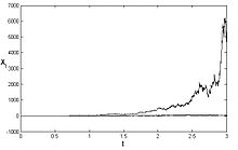
See numerical solution is presented above for three different trajectories.^[4]

Numerical solution for the stochastic differential equation just presented, the drift is twice the diffusion coefficient.

Computer implementation[]

The following Python code implements the Milstein method and uses it to solve the SDE describing the Geometric Brownian Motion defined by

${\displaystyle dY_{t}=\,\mu Y\,{\mathrm {d} }t+\sigma Y\,{\mathrm {d} }W_{t}}$

${\displaystyle Y_{0}=Y_{\mathrm {init} }}$

# -*- coding: utf-8 -*-
# Milstein Method

import numpy as np
import matplotlib.pyplot as plt

num_sims = 1  # One Example

# One Second and thousand grid points
t_init = 0
t_end  = 1
N      = 1000 # Compute 1000 grid points
dt     = float(t_end - t_init) / N

## Initial Conditions
y_init = 1
mu    = 3
sigma = 1


# dw Random process
def dW(delta_t):
    """Random sample normal distribution"""
    return np.random.normal(loc=0.0, scale=np.sqrt(delta_t))

# vectors to fill
ts = np.arange(t_init, t_end + dt, dt)
ys = np.zeros(N + 1)
ys[0] = y_init

# Loop
for _ in range(num_sims):
    for i in range(1, ts.size):
        t = (i - 1) * dt
        y = ys[i - 1]
        # Milstein method
        ys[i] = y + mu * dt * y + sigma* y* dW(dt) + 0.5* sigma**2 * y* (dW(dt)**2 - dt)
    plt.plot(ts, ys)

# Plot
plt.xlabel("time (s)")
plt.grid()
h = plt.ylabel("y")
h.set_rotation(0)
plt.show()

See also[]

• Euler–Maruyama method

References[]

Further reading[]

• Kloeden, P.E., & Platen, E. (1999). Numerical Solution of Stochastic Differential Equations. Springer, Berlin. ISBN 3-540-54062-8.CS1 maint: multiple names: authors list (link)