Queueing theory

Queue networks are systems in which single queues are connected by a routing network. In this image, servers are represented by circles, queues by a series of rectangles and the routing network by arrows. In the study of queue networks one typically tries to obtain the equilibrium distribution of the network, although in many applications the study of the transient state is fundamental.

Queueing theory is the mathematical study of waiting lines, or queues.^[1] A queueing model is constructed so that queue lengths and waiting time can be predicted.^[1] Queueing theory is generally considered a branch of operations research because the results are often used when making business decisions about the resources needed to provide a service.

Queueing theory has its origins in research by Agner Krarup Erlang when he created models to describe the system of Copenhagen Telephone Exchange company, a Danish company.^[1] The ideas have since seen applications including telecommunication, traffic engineering, computing^[2] and, particularly in industrial engineering, in the design of factories, shops, offices and hospitals, as well as in project management.^[3][4]

Spelling[]

The spelling "queueing" over "queuing" is typically encountered in the academic research field. In fact, one of the flagship journals of the field is Queueing Systems.

Single queueing nodes[]

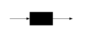
A queue, or queueing node can be thought of as nearly a black box. Jobs or "customers" arrive to the queue, possibly wait some time, take some time being processed, and then depart from the queue.

A black box. Jobs arrive to, and depart from, the queue.

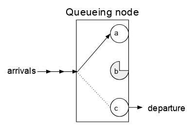
The queueing node is not quite a pure black box, however, since some information is needed about the inside of the queuing node. The queue has one or more "servers" which can each be paired with an arriving job until it departs, after which that server will be free to be paired with another arriving job.

A queueing node with 3 servers. Server a is idle, and thus an arrival is given to it to process. Server b is currently busy and will take some time before it can complete service of its job. Server c has just completed service of a job and thus will be next to receive an arriving job.

An analogy often used is that of the cashier at a supermarket. There are other models, but this is one commonly encountered in the literature. Customers arrive, are processed by the cashier, and depart. Each cashier processes one customer at a time, and hence this is a queueing node with only one server. A setting where a customer will leave immediately if the cashier is busy when the customer arrives, is referred to as a queue with no buffer (or no "waiting area", or similar terms). A setting with a waiting zone for up to n customers is called a queue with a buffer of size n.

Birth-death process[]

The behaviour of a single queue (also called a "queueing node") can be described by a birth–death process, which describes the arrivals and departures from the queue, along with the number of jobs (also called "customers" or "requests", or any number of other things, depending on the field) currently in the system. An arrival increases the number of jobs by 1, and a departure (a job completing its service) decreases k by 1.

A birth–death process. The values in the circles represent the state of the birth-death process. For a queueing system, k is the number of jobs in the system (either being serviced or waiting if the queue has a buffer of waiting jobs). The system transitions between values of k by "births" and "deaths" which occur at rates given by various values of λ_i and μ_i, respectively. Further, for a queue, the arrival rates and departure rates are generally considered not to vary with the number of jobs in the queue, so a single average rate of arrivals/departures per unit time to the queue is assumed. Under this assumption, this process has an arrival rate of λ = λ₁, λ₂, ..., λ_k and a departure rate of μ = μ₁, μ₂, ..., μ_k (see next figure).

A queue with 1 server, arrival rate λ and departure rate μ.

Balance equations[]

The steady state equations for the birth-and-death process, known as the balance equations, are as follows. Here ${\displaystyle P_{n}}$ denotes the steady state probability to be in state n.

${\displaystyle \mu _{1}P_{1}=\lambda _{0}P_{0}}$

${\displaystyle \lambda _{0}P_{0}+\mu _{2}P_{2}=(\lambda _{1}+\mu _{1})P_{1}}$

${\displaystyle \lambda _{n-1}P_{n-1}+\mu _{n+1}P_{n+1}=(\lambda _{n}+\mu _{n})P_{n}}$

The first two equations imply

${\displaystyle P_{1}={\frac {\lambda _{0}}{\mu _{1}}}P_{0}}$

and

${\displaystyle P_{2}={\frac {\lambda _{1}}{\mu _{2}}}P_{1}+{\frac {1}{\mu _{2}}}(\mu _{1}P_{1}-\lambda _{0}P_{0})={\frac {\lambda _{1}}{\mu _{2}}}P_{1}={\frac {\lambda _{1}\lambda _{0}}{\mu _{2}\mu _{1}}}P_{0}.}$

By mathematical induction,

${\displaystyle P_{n}={\frac {\lambda _{n-1}\lambda _{n-2}\cdots \lambda _{0}}{\mu _{n}\mu _{n-1}\cdots \mu _{1}}}P_{0}=P_{0}\prod _{i=0}^{n-1}{\frac {\lambda _{i}}{\mu _{i+1}}}.}$

The condition ${\displaystyle \sum _{n=0}^{\infty }P_{n}=P_{0}+P_{0}\sum _{n=1}^{\infty }\prod _{i=0}^{n-1}{\frac {\lambda _{i}}{\mu _{i+1}}}=1}$ leads to:

${\displaystyle P_{0}={\frac {1}{1+\sum _{n=1}^{\infty }\prod _{i=0}^{n-1}{\frac {\lambda _{i}}{\mu _{i+1}}}}},}$

which, together with the equation for ${\displaystyle P_{n}}$ ${\displaystyle (n\geq 1)}$, fully describes the required steady state probabilities.

Kendall's notation[]

Single queueing nodes are usually described using Kendall's notation in the form A/S/c where A describes the distribution of durations between each arrival to the queue, S the distribution of service times for jobs and c the number of servers at the node.^[5][6] For an example of the notation, the M/M/1 queue is a simple model where a single server serves jobs that arrive according to a Poisson process (where inter-arrival durations are exponentially distributed) and have exponentially distributed service times (the M denotes a Markov process). In an M/G/1 queue, the G stands for "general" and indicates an arbitrary probability distribution for service times.

Example analysis of an M/M/1 queue[]

Consider a queue with one server and the following characteristics:

• λ: the arrival rate (the reciprocal of the expected time between each customer arriving, e.g. 10 customers per second);
• μ: the reciprocal of the mean service time (the expected number of consecutive service completions per the same unit time, e.g. per 30 seconds);
• n: the parameter characterizing the number of customers in the system;
• P_n: the probability of there being n customers in the system in steady state.

Further, let E_n represent the number of times the system enters state n, and L_n represent the number of times the system leaves state n. Then for all n, |E_n − L_n| ∈ {0, 1}. That is, the number of times the system leaves a state differs by at most 1 from the number of times it enters that state, since it will either return into that state at some time in the future (E_n = L_n) or not (|E_n − L_n| = 1).

When the system arrives at a steady state, the arrival rate should be equal to the departure rate.

Thus the balance equations

${\displaystyle \mu P_{1}=\lambda P_{0}}$

${\displaystyle \lambda P_{0}+\mu P_{2}=(\lambda +\mu )P_{1}}$

${\displaystyle \lambda P_{n-1}+\mu P_{n+1}=(\lambda +\mu )P_{n}}$

imply

${\displaystyle P_{n}={\frac {\lambda }{\mu }}P_{n-1},\ n=1,2,\ldots }$

The fact that ${\displaystyle P_{0}+P_{1}+\cdots =1}$ leads to the geometric distribution formula

${\displaystyle P_{n}=(1-\rho )\rho ^{n}}$

where ${\displaystyle \rho ={\frac {\lambda }{\mu }}<1.}$

Simple two-equation queue[]

A common basic queuing system is attributed to Erlang, and is a modification of Little's Law. Given an arrival rate λ, a dropout rate σ, and a departure rate μ, length of the queue L is defined as:

${\displaystyle L={\frac {\lambda -\sigma }{\mu }}.}$

Assuming an exponential distribution for the rates, the waiting time W can be defined as the proportion of arrivals that are served. This is equal to the exponential survival rate of those who do not drop out over the waiting period, giving:

${\displaystyle {\frac {\mu }{\lambda }}=e^{-W{\mu }}}$

The second equation is commonly rewritten as:

${\displaystyle W={\frac {1}{\mu }}\mathrm {ln} {\frac {\lambda }{\mu }}}$

The two-stage one-box model is common in epidemiology.^[7]

Overview of the development of the theory[]

In 1909, Agner Krarup Erlang, a Danish engineer who worked for the Copenhagen Telephone Exchange, published the first paper on what would now be called queueing theory.^[8][9][10] He modeled the number of telephone calls arriving at an exchange by a Poisson process and solved the M/D/1 queue in 1917 and M/D/k queueing model in 1920.^[11] In Kendall's notation:

• M stands for Markov or memoryless and means arrivals occur according to a Poisson process;
• D stands for deterministic and means jobs arriving at the queue which require a fixed amount of service;
• k describes the number of servers at the queueing node (k = 1, 2, ...).

If there are more jobs at the node than there are servers, then jobs will queue and wait for service

The M/G/1 queue was solved by Felix Pollaczek in 1930,^[12] a solution later recast in probabilistic terms by Aleksandr Khinchin and now known as the Pollaczek–Khinchine formula.^[11][13]

After the 1940s queueing theory became an area of research interest to mathematicians.^[13] In 1953 David George Kendall solved the GI/M/k queue^[14] and introduced the modern notation for queues, now known as Kendall's notation. In 1957 Pollaczek studied the GI/G/1 using an integral equation.^[15] John Kingman gave a formula for the mean waiting time in a G/G/1 queue: Kingman's formula.^[16]

Leonard Kleinrock worked on the application of queueing theory to message switching in the early 1960s and packet switching in the early 1970s. His initial contribution to this field was his doctoral thesis at the Massachusetts Institute of Technology in 1962, published in book form in 1964. His theoretical work published in the early 1970s underpinned the use of packet switching in the ARPANET, a forerunner to the Internet.

The matrix geometric method and matrix analytic methods have allowed queues with phase-type distributed inter-arrival and service time distributions to be considered.^[17]

Systems with coupled orbits are an important part in queueing theory in the application to wireless networks and signal processing. ^[18]

Problems such as performance metrics for the M/G/k queue remain an open problem.^[11][13]

Service disciplines[]

First in first out (FIFO) queue example.

Various scheduling policies can be used at queuing nodes:

First in first out

Also called first-come, first-served (FCFS),^[19] this principle states that customers are served one at a time and that the customer that has been waiting the longest is served first.^[20]

Last in first out

This principle also serves customers one at a time, but the customer with the shortest waiting time will be served first.^[20] Also known as a stack.

Processor sharing

Service capacity is shared equally between customers.^[20]

Priority

Customers with high priority are served first.^[20] Priority queues can be of two types, non-preemptive (where a job in service cannot be interrupted) and preemptive (where a job in service can be interrupted by a higher-priority job). No work is lost in either model.^[21]

Shortest job first

The next job to be served is the one with the smallest size^[22]

Preemptive shortest job first

The next job to be served is the one with the original smallest size^[23]

Shortest remaining processing time

The next job to serve is the one with the smallest remaining processing requirement.^[24]

Service facility

• Single server: customers line up and there is only one server
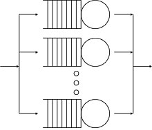
• Several parallel servers–Single queue: customers line up and there are several servers
• Several servers–Several queues: there are many counters and customers can decide going where to queue

Unreliable server

Server failures occur according to a stochastic process (usually Poisson) and are followed by the setup periods during which the server is unavailable. The interrupted customer remains in the service area until server is fixed.^[25]

Customer's behavior of waiting

• Balking: customers deciding not to join the queue if it is too long
• Jockeying: customers switch between queues if they think they will get served faster by doing so
• Reneging: customers leave the queue if they have waited too long for service

Arriving customers not served (either due to the queue having no buffer, or due to balking or reneging by the customer) are also known as dropouts and the average rate of dropouts is a significant parameter describing a queue.

Queueing networks[]

Networks of queues are systems in which a number of queues are connected by what's known as customer routing. When a customer is serviced at one node it can join another node and queue for service, or leave the network.

For networks of m nodes, the state of the system can be described by an m–dimensional vector (x₁, x₂, ..., x_m) where x_i represents the number of customers at each node.

The simplest non-trivial network of queues is called tandem queues.^[26] The first significant results in this area were Jackson networks,^[27][28] for which an efficient product-form stationary distribution exists and the mean value analysis^[29] which allows average metrics such as throughput and sojourn times to be computed.^[30] If the total number of customers in the network remains constant the network is called a closed network and has also been shown to have a product–form stationary distribution in the Gordon–Newell theorem.^[31] This result was extended to the BCMP network^[32] where a network with very general service time, regimes and customer routing is shown to also exhibit a product-form stationary distribution. The normalizing constant can be calculated with the Buzen's algorithm, proposed in 1973.^[33]

Networks of customers have also been investigated, Kelly networks where customers of different classes experience different priority levels at different service nodes.^[34] Another type of network are G-networks first proposed by Erol Gelenbe in 1993:^[35] these networks do not assume exponential time distributions like the classic Jackson Network.

Routing algorithms[]

In discrete time networks where there is a constraint on which service nodes can be active at any time, the max-weight scheduling algorithm chooses a service policy to give optimal throughput in the case that each job visits only a single person ^[19] service node. In the more general case where jobs can visit more than one node, backpressure routing gives optimal throughput. A network scheduler must choose a queuing algorithm, which affects the characteristics of the larger network^{[citation needed]}. See also Stochastic scheduling for more about scheduling of queueing systems.

Mean field limits[]

Mean field models consider the limiting behaviour of the empirical measure (proportion of queues in different states) as the number of queues (m above) goes to infinity. The impact of other queues on any given queue in the network is approximated by a differential equation. The deterministic model converges to the same stationary distribution as the original model.^[36]

Heavy traffic/diffusion approximations[]

In a system with high occupancy rates (utilisation near 1) a heavy traffic approximation can be used to approximate the queueing length process by a reflected Brownian motion,^[37] Ornstein–Uhlenbeck process, or more general diffusion process.^[38] The number of dimensions of the Brownian process is equal to the number of queueing nodes, with the diffusion restricted to the non-negative orthant.

Fluid limits[]

Fluid models are continuous deterministic analogs of queueing networks obtained by taking the limit when the process is scaled in time and space, allowing heterogeneous objects. This scaled trajectory converges to a deterministic equation which allows the stability of the system to be proven. It is known that a queueing network can be stable, but have an unstable fluid limit.^[39]

Softwarized Network Services[]

When we use softwarized network services in a queueing network, we find that measuring the different times of response of our network is a important thing because it might affect all our system. Knowing those data and trying to correct those that can cause an error is a task that we have to solve.^[40]

See also[]

References[]

Further reading[]

• Gross, Donald; Carl M. Harris (1998). Fundamentals of Queueing Theory. Wiley. ISBN 978-0-471-32812-4. Online
• Zukerman, Moshe (2013). Introduction to Queueing Theory and Stochastic Teletraffic Models (PDF). arXiv:1307.2968.
• Deitel, Harvey M. (1984) [1982]. An introduction to operating systems (revisited first ed.). Addison-Wesley. p. 673. ISBN 978-0-201-14502-1. chap.15, pp. 380–412
• Gelenbe, Erol; Isi Mitrani (2010). Analysis and Synthesis of Computer Systems. World Scientific 2nd Edition. ISBN 978-1-908978-42-4.
• Newell, Gordron F. (1 June 1971). Applications of Queueing Theory. Chapman and Hall.
• Leonard Kleinrock, Information Flow in Large Communication Nets, (MIT, Cambridge, May 31, 1961) Proposal for a Ph.D. Thesis
• Leonard Kleinrock. Information Flow in Large Communication Nets (RLE Quarterly Progress Report, July 1961)
• Leonard Kleinrock. Communication Nets: Stochastic Message Flow and Delay (McGraw-Hill, New York, 1964)
• Kleinrock, Leonard (2 January 1975). Queueing Systems: Volume I – Theory. New York: Wiley Interscience. pp. 417. ISBN 978-0471491101.
• Kleinrock, Leonard (22 April 1976). Queueing Systems: Volume II – Computer Applications. New York: Wiley Interscience. pp. 576. ISBN 978-0471491118.
• Lazowska, Edward D.; John Zahorjan; G. Scott Graham; Kenneth C. Sevcik (1984). Quantitative System Performance: Computer System Analysis Using Queueing Network Models. Prentice-Hall, Inc. ISBN 978-0-13-746975-8.
• Jon Kleinberg; Éva Tardos (30 June 2013). Algorithm Design. Pearson. ISBN 978-1-292-02394-6.

External links[]

Look up queueing or queuing in Wiktionary, the free dictionary.

This article's use of external links may not follow Wikipedia's policies or guidelines. Please by removing excessive or inappropriate external links, and converting useful links where appropriate into footnote references. (May 2017) (Learn how and when to remove this template message)

• Queueing theory calculator
• Teknomo's Queueing theory tutorial and calculators
• Office Fire Emergency Evacuation Simulation on YouTube
• Virtamo's Queueing Theory Course
• Myron Hlynka's Queueing Theory Page
• Queueing Theory Basics
• A free online tool to solve some classical queueing systems
• JMT: an open source graphical environment for queueing theory
• LINE: a general-purpose engine to solve queueing models
• What You Hate Most About Waiting in Line: (It’s not the length of the wait.), by Seth Stevenson, Slate, 2012 – popular introduction