Probability distribution

Part of a series on statistics
Probability theory
Probability Axioms Determinism System Indeterminism Randomness
Probability space Sample space Event Collectively exhaustive events Elementary event Mutual exclusivity Outcome Singleton Experiment Bernoulli trial Probability distribution Bernoulli distribution Binomial distribution Normal distribution Probability measure Random variable Bernoulli process Continuous or discrete Expected value Markov chain Observed value Random walk Stochastic process
Complementary event Joint probability Marginal probability Conditional probability
Independence Conditional independence Law of total probability Law of large numbers Bayes' theorem Boole's inequality
Venn diagram Tree diagram
v t

In probability theory and statistics, a probability distribution is the mathematical function that gives the probabilities of occurrence of different possible outcomes for an experiment.^[1][2] It is a mathematical description of a random phenomenon in terms of its sample space and the probabilities of events (subsets of the sample space).^[3]

For instance, if X is used to denote the outcome of a coin toss ("the experiment"), then the probability distribution of X would take the value 0.5 (1 in 2 or 1/2) for X = heads, and 0.5 for X = tails (assuming that the coin is fair). Examples of random phenomena include the weather condition in a future date, the height of a randomly selected person, the fraction of male students in a school, the results of a survey to be conducted, etc.^[4]

Introduction[]

The probability mass function (pmf) p(S) specifies the probability distribution for the sum S of counts from two dice. For example, the figure shows that p(11) = 2/36 = 1/18. The pmf allows the computation of probabilities of events such as P(S > 9) = 1/12 + 1/18 + 1/36 = 1/6, and all other probabilities in the distribution.

A probability distribution is a mathematical description of the probabilities of events, subsets of the sample space. The sample space, often denoted by ${\displaystyle \Omega }$,^[5] is the set of all possible outcomes of a random phenomenon being observed; it may be any set: a set of real numbers, a set of vectors, a set of arbitrary non-numerical values, etc. For example, the sample space of a coin flip would be Ω = {heads, tails}.

To define probability distributions for the specific case of random variables (so the sample space can be seen as a numeric set), it is common to distinguish between discrete and continuous random variables. In the discrete case, it is sufficient to specify a probability mass function ${\displaystyle p}$ assigning a probability to each possible outcome: for example, when throwing a fair die, each of the six values 1 to 6 has the probability 1/6. The probability of an event is then defined to be the sum of the probabilities of the outcomes that satisfy the event; for example, the probability of the event "the die rolls an even value" is

${\displaystyle p(2)+p(4)+p(6)=1/6+1/6+1/6=1/2.}$

In contrast, when a random variable takes values from a continuum then typically, any individual outcome has probability zero and only events that include infinitely many outcomes, such as intervals, can have positive probability. For example, consider measuring the weight of a piece of ham in the supermarket, and assume the scale has many digits of precision. The probability that it weighs exactly 500 g is zero, as it will most likely have some non-zero decimal digits. Nevertheless, one might demand, in quality control, that a package of "500 g" of ham must weigh between 490 g and 510 g with at least 98% probability, and this demand is less sensitive to the accuracy of measurement instruments.

On the left is the probability density function. On the right is the cumulative distribution function, which is the area under the probability density curve.

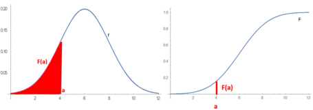
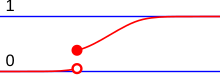
Continuous probability distributions can be described in several ways. The probability density function describes the infinitesimal probability of any given value, and the probability that the outcome lies in a given interval can be computed by integrating the probability density function over that interval.^[6] An alternative description of the distribution is by means of the cumulative distribution function, which describes the probability that the random variable is no larger than a given value (i.e., P(X < x) for some x). The cumulative distribution function is the area under the probability density function from ${\displaystyle -\infty }$ to x, as described by the picture to the right.^[7]

General definition[]

A probability distribution can be described in various forms, such as by a probability mass function or a cumulative distribution function. One of the most general descriptions, which applies for continuous and discrete variables, is by means of a probability function ${\displaystyle P\colon {\mathcal {A}}\rightarrow \mathbb {R} }$ whose input space ${\displaystyle {\mathcal {A}}}$ is related to the sample space, and gives a probability as its output.^[8]

The probability function P can take as argument subsets of the sample space itself, as in the coin toss example, where the function P was defined so that P(heads) = 0.5 and P(tails) = 0.5. However, because of the widespread use of random variables, which transform the sample space into a set of numbers (e.g., ${\displaystyle \mathbb {R} }$, ${\displaystyle \mathbb {N} }$), it is more common to study probability distributions whose argument are subsets of these particular kinds of sets (number sets),^[9] and all probability distributions discussed in this article are of this type. It is common to denote as P(X ${\displaystyle \in }$ E) the probability that a certain variable X belongs to a certain event E.^[4][10]

The above probability function only characterizes a probability distribution if it satisfies all the Kolmogorov axioms, that is:

1. ${\displaystyle P(X\in E)\geq 0\;\forall E\in {\mathcal {A}}}$, so the probability is non-negative
2. ${\displaystyle P(X\in E)\leq 1\;\forall E\in {\mathcal {A}}}$, so no probability exceeds ${\displaystyle 1}$
3. ${\displaystyle P(X\in \bigsqcup _{i}E_{i})=\sum _{i}P(X\in E_{i})}$ for any disjoint family of sets ${\displaystyle \{E_{i}\}}$

The concept of probability function is made more rigorous by defining it as the element of a probability space ${\displaystyle (X,{\mathcal {A}},P)}$, where ${\displaystyle X}$ is the set of possible outcomes, ${\displaystyle {\mathcal {A}}}$ is the set of all subsets ${\displaystyle E\subset X}$ whose probability can be measured, and ${\displaystyle P}$ is the probability function, or probability measure, that assigns a probability to each of these measurable subsets ${\displaystyle E\in {\mathcal {A}}}$.^[11]

Probability distributions are generally divided into two classes. A discrete probability distribution is applicable to the scenarios where the set of possible outcomes is discrete (e.g. a coin toss, a roll of a die) and the probabilities are encoded by a discrete list of the probabilities of the outcomes; in this case the discrete probability distribution is known as probability mass function. On the other hand, continuous probability distributions are applicable to scenarios where the set of possible outcomes can take on values in a continuous range (e.g. real numbers), such as the temperature on a given day. In the case of real numbers, the continuous probability distribution is the cumulative distribution function. In general, in the continuous case, probabilities are described by a probability density function, and the probability distribution is by definition the integral of the probability density function.^[4][6][10] The normal distribution is a commonly encountered continuous probability distribution. More complex experiments, such as those involving stochastic processes defined in continuous time, may demand the use of more general probability measures.

A probability distribution whose sample space is one-dimensional (for example real numbers, list of labels, ordered labels or binary) is called univariate, while a distribution whose sample space is a vector space of dimension 2 or more is called multivariate. A univariate distribution gives the probabilities of a single random variable taking on various different values; a multivariate distribution (a joint probability distribution) gives the probabilities of a random vector – a list of two or more random variables – taking on various combinations of values. Important and commonly encountered univariate probability distributions include the binomial distribution, the hypergeometric distribution, and the normal distribution. A commonly encountered multivariate distribution is the multivariate normal distribution.

Besides the probability function, the cumulative distribution function, the probability mass function and the probability density function, the moment generating function and the characteristic function also serve to identify a probability distribution, as they uniquely determine an underlying cumulative distribution function.^[12]

The probability density function (pdf) of the normal distribution, also called Gaussian or "bell curve", the most important continuous random distribution. As notated on the figure, the probabilities of intervals of values correspond to the area under the curve.

Terminology[]

Some key concepts and terms, widely used in the literature on the topic of probability distributions, are listed below.^[1]

Functions for discrete variables[]

• Probability function: describes the probability ${\displaystyle P(X\in E)}$ that the event ${\displaystyle E,}$ from the sample space occurs.^[8]
• Probability mass function (pmf): function that gives the probability that a discrete random variable is equal to some value.
• Frequency distribution: a table that displays the frequency of various outcomes in a sample.
• Relative frequency distribution: a frequency distribution where each value has been divided (normalized) by a number of outcomes in a sample (i.e. sample size).
• Discrete probability distribution function: general term to indicate the way the total probability of 1 is distributed over all various possible outcomes (i.e. over entire population) for discrete random variable.
• Cumulative distribution function: function evaluating the probability that ${\displaystyle X}$ will take a value less than or equal to ${\displaystyle x}$ for a discrete random variable.
• Categorical distribution: for discrete random variables with a finite set of values.

Functions for continuous variables[]

• Probability density function (pdf): function whose value at any given sample (or point) in the sample space (the set of possible values taken by the random variable) can be interpreted as providing a relative likelihood that the value of the random variable would equal that sample.
• Continuous probability distribution function: most often reserved for continuous random variables.
• Cumulative distribution function: function evaluating the probability that ${\displaystyle X}$ will take a value less than or equal to ${\displaystyle x}$ for a continuous variable.
• Quantile function: the inverse of the cumulative distribution function. Gives ${\displaystyle x}$ such that, with probability ${\displaystyle q}$, ${\displaystyle X}$ will not exceed ${\displaystyle x}$.

Basic terms[]

• Mode: for a discrete random variable, the value with highest probability; for a continuous random variable, a location at which the probability density function has a local peak.
• Support: set of values that can be assumed with non-zero probability by the random variable. For a random variable ${\displaystyle X}$, it is sometimes denoted as ${\displaystyle R_{X}}$.^[5]
• Tail:^[13] the regions close to the bounds of the random variable, if the pmf or pdf are relatively low therein. Usually has the form ${\displaystyle X>a}$, ${\displaystyle X<b}$ or a union thereof.
• Head:^[13] the region where the pmf or pdf is relatively high. Usually has the form ${\displaystyle a<X<b}$.
• Expected value or mean: the weighted average of the possible values, using their probabilities as their weights; or the continuous analog thereof.
• Median: the value such that the set of values less than the median, and the set greater than the median, each have probabilities no greater than one-half.
• Variance: the second moment of the pmf or pdf about the mean; an important measure of the dispersion of the distribution.
• Standard deviation: the square root of the variance, and hence another measure of dispersion.
• Quantile: the q-quantile is the value ${\displaystyle x}$ such that ${\displaystyle P(X<x)=q}$.
• Symmetry: a property of some distributions in which the portion of the distribution to the left of a specific value (usually the median) is a mirror image of the portion to its right.
• Skewness: a measure of the extent to which a pmf or pdf "leans" to one side of its mean. The third standardized moment of the distribution.
• Kurtosis: a measure of the "fatness" of the tails of a pmf or pdf. The fourth standardized moment of the distribution.

Discrete probability distribution[]

The probability mass function of a discrete probability distribution. The probabilities of the singletons {1}, {3}, and {7} are respectively 0.2, 0.5, 0.3. A set not containing any of these points has probability zero.

The cdf of a discrete probability distribution, ...

... of a continuous probability distribution, ...

... of a distribution which has both a continuous part and a discrete part.

A discrete probability distribution is the probability distribution of a random variable that can take on only a countable number of values.^[14] In the case where the range of values is countably infinite, these values have to decline to zero fast enough for the probabilities to add up to 1. For example, if ${\displaystyle \operatorname {P} (X=n)={\tfrac {1}{2^{n}}}}$ for n = 1, 2, ..., the sum of probabilities would be 1/2 + 1/4 + 1/8 + ... = 1.

Well-known discrete probability distributions used in statistical modeling include the Poisson distribution, the Bernoulli distribution, the binomial distribution, the geometric distribution, and the negative binomial distribution.^[3] Additionally, the discrete uniform distribution is commonly used in computer programs that make equal-probability random selections between a number of choices.

When a sample (a set of observations) is drawn from a larger population, the sample points have an empirical distribution that is discrete, and which provides information about the population distribution.

Cumulative distribution function[]

Equivalently to the above, a discrete random variable can be defined as a random variable whose cumulative distribution function (cdf) increases only by jump discontinuities—that is, its cdf increases only where it "jumps" to a higher value, and is constant between those jumps. Note however that the points where the cdf jumps may form a dense set of the real numbers. The points where jumps occur are precisely the values which the random variable may take.

Delta-function representation[]

Consequently, a discrete probability distribution is often represented as a generalized probability density function involving Dirac delta functions, which substantially unifies the treatment of continuous and discrete distributions. This is especially useful when dealing with probability distributions involving both a continuous and a discrete part.^[15]

Indicator-function representation[]

For a discrete random variable X, let u₀, u₁, ... be the values it can take with non-zero probability. Denote

${\displaystyle \Omega _{i}=X^{-1}(u_{i})=\{\omega :X(\omega )=u_{i}\},\,i=0,1,2,\dots }$

These are disjoint sets, and for such sets

${\displaystyle P\left(\bigcup _{i}\Omega _{i}\right)=\sum _{i}P(\Omega _{i})=\sum _{i}P(X=u_{i})=1.}$

It follows that the probability that X takes any value except for u₀, u₁, ... is zero, and thus one can write X as

${\displaystyle X(\omega )=\sum _{i}u_{i}1_{\Omega _{i}}(\omega )}$

except on a set of probability zero, where ${\displaystyle 1_{A}}$ is the indicator function of A. This may serve as an alternative definition of discrete random variables.

One-point distribution[]

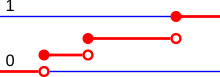
A special case is the discrete distribution of a random variable that can take on only one fixed value; in other words, it is a deterministic distribution. Expressed formally, the random variable ${\displaystyle X}$ has a one-point distribution if it has a possible outcome ${\displaystyle x}$ such that ${\displaystyle P(X{=}x)=1.}$^[16] All other possible outcomes then have probability 0. Its cumulative distribution function jumps immediately from 0 to 1.

Continuous probability distribution[]

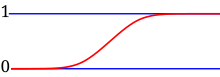
A continuous probability distribution is a probability distribution whose support is an uncountable set, such as an interval in the real line.^[17] They are uniquely characterized by a cumulative distribution function that can be used to calculate the probability for each subset of the support. There are many examples of continuous probability distributions: normal, uniform, chi-squared, and others.

A random variable ${\displaystyle X}$ has a continuous probability distribution if there is a function ${\displaystyle f:\mathbb {R} \rightarrow [0,\infty ]}$ such that for each interval ${\displaystyle I\subset \mathbb {R} }$ the probability of ${\displaystyle X}$ belonging to ${\displaystyle I}$ is given by the integral of ${\displaystyle f}$ over ${\displaystyle I}$.^[18] For example, if ${\displaystyle I=[a,b]}$, then we would have:^[19]

${\displaystyle \operatorname {P} \left[a\leq X\leq b\right]=\int _{a}^{b}f(x)\,dx}$

In particular, the probability for ${\displaystyle X}$ to take any single value ${\displaystyle a}$ (that is, ${\displaystyle a\leq X\leq a}$) is zero, because an integral with coinciding upper and lower limits is always equal to zero. A variable that satisfies the above is called continuous random variable. Its cumulative density function is defined as

${\displaystyle F(x)=\operatorname {P} \left[-\infty <X\leq x\right]=\int _{-\infty }^{x}f(x)\,dx}$

which, by this definition, has the properties:

• ${\displaystyle F(x)}$ is non-decreasing;
• ${\displaystyle 0\leq F(x)\leq 1}$;
• ${\displaystyle \lim _{x\rightarrow -\infty }F(x)=0}$ and ${\displaystyle \lim _{x\rightarrow \infty }F(x)=1}$;
• ${\displaystyle \operatorname {P} (a<X\leq b)=F(b)-F(a)}$; and
• ${\displaystyle F(x)}$ is continuous due to the Riemann integral properties.^[20]

It is also possible to think in the opposite direction, which allows more flexibility: if ${\displaystyle F(x)}$ is a function that satisfies all but the last of the properties above, then ${\displaystyle F}$ represents the cumulative density function for some random variable: a discrete random variable if ${\displaystyle F}$ is a step function, and a continuous random variable otherwise.^[21] This allows for continuous distributions that have a cumulative density function, but not a probability density function, such as the Cantor distribution.

It is often necessary to generalize the above definition for more arbitrary subsets of the real line. In these contexts, a continuous probability distribution is defined as a probability distribution with a cumulative distribution function that is absolutely continuous. Equivalently, it is a probability distribution on the real numbers that is absolutely continuous with respect to the Lebesgue measure. Such distributions can be represented by their probability density functions. If ${\displaystyle X}$ is such an absolutely continuous random variable, then it has a probability density function ${\displaystyle f(x)}$, and its probability of falling into a Lebesgue-measurable set ${\displaystyle A\subset \mathbb {R} }$ is:

${\displaystyle \operatorname {P} \left[X\in A\right]=\int _{A}f(x)\,d\mu }$

where ${\displaystyle \mu }$ is the Lebesgue measure.

Note on terminology: some authors use the term "continuous distribution" to denote distributions whose cumulative distribution functions are continuous, rather than absolutely continuous. These distributions are the ones ${\displaystyle \mu }$ such that ${\displaystyle \mu \{x\}\,=\,0}$ for all ${\displaystyle \,x}$. This definition includes the (absolutely) continuous distributions defined above, but it also includes singular distributions, which are neither absolutely continuous nor discrete nor a mixture of those, and do not have a density. An example is given by the Cantor distribution.

Kolmogorov definition[]

In the measure-theoretic formalization of probability theory, a random variable is defined as a measurable function ${\displaystyle X}$ from a probability space ${\displaystyle (\Omega ,{\mathcal {F}},\mathbb {P} )}$ to a measurable space ${\displaystyle ({\mathcal {X}},{\mathcal {A}})}$. Given that probabilities of events of the form ${\displaystyle \{\omega \in \Omega \mid X(\omega )\in A\}}$ satisfy Kolmogorov's probability axioms, the probability distribution of X is the pushforward measure ${\displaystyle X_{*}\mathbb {P} }$ of ${\displaystyle X}$ , which is a probability measure on ${\displaystyle ({\mathcal {X}},{\mathcal {A}})}$ satisfying ${\displaystyle X_{*}\mathbb {P} =\mathbb {P} X^{-1}}$.^[22][23][24]

Other kinds of distributions[]

One solution for the Rabinovich–Fabrikant equations. What is the probability of observing a state on a certain place of the support (i.e., the red subset)?

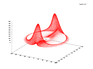
Continuous and discrete distributions with support on ${\displaystyle \mathbb {R} ^{k}}$ or ${\displaystyle \mathbb {N} ^{k}}$ are extremely useful to model a myriad of phenomena,^[4][7] since most practical distributions are supported on relatively simple subsets, such as hypercubes or balls. However, this is not always the case, and there exist phenomena with supports that are actually complicated curves ${\displaystyle \gamma :[a,b]\rightarrow \mathbb {R} ^{n}}$ within some space ${\displaystyle \mathbb {R} ^{n}}$ or similar. In these cases, the probability distribution is supported on the image of such curve, and is likely to be determined empirically, rather than finding a closed formula for it.^[25]

One example is shown in the figure to the right, which displays the evolution of a system of differential equations (commonly known as the Rabinovich–Fabrikant equations) that can be used to model the behaviour of Langmuir waves in plasma.^[26] When this phenomenon is studied, the observed states from the subset are as indicated in red. So one could ask what is the probability of observing a state in a certain position of the red subset; if such a probability exists, it is called the probability measure of the system.^[27][25]

This kind of complicated support appears quite frequently in dynamical systems. It is not simple to establish that the system has a probability measure, and the main problem is the following. Let ${\displaystyle t_{1}\ll t_{2}\ll t_{3}}$ be instants in time and ${\displaystyle O}$ a subset of the support; if the probability measure exists for the system, one would expect the frequency of observing states inside set ${\displaystyle O}$ would be equal in interval ${\displaystyle [t_{1},t_{2}]}$ and ${\displaystyle [t_{2},t_{3}]}$, which might not happen; for example, it could oscillate similar to a sine, ${\displaystyle \sin(t)}$, whose limit when ${\displaystyle t\rightarrow \infty }$ does not converge. Formally, the measure exists only if the limit of the relative frequency converges when the system is observed into the infinite future.^[28] The branch of dynamical systems that studies the existence of a probability measure is ergodic theory.

Note that even in these cases, the probability distribution, if it exists, might still be termed "continuous" or "discrete" depending on whether the support is uncountable or countable, respectively.

Random number generation[]

Most algorithms are based on a pseudorandom number generator that produces numbers X that are uniformly distributed in the half-open interval [0,1). These random variates X are then transformed via some algorithm to create a new random variate having the required probability distribution. With this source of uniform pseudo-randomness, realizations of any random variable can be generated.^[29]

For example, suppose ${\displaystyle U}$ has a uniform distribution between 0 and 1. To construct a random Bernoulli variable for some ${\displaystyle 0<p<1}$, we define

${\displaystyle {\displaystyle X={\begin{cases}1,&{\mbox{if }}U<p\\0,&{\mbox{if }}U\geq p\end{cases}}}}$

so that

${\displaystyle {\textrm {P}}(X=1)={\textrm {P}}(U<p)=p,{\textrm {P}}(X=0)={\textrm {P}}(U\geq p)=1-p.}$

This random variable X has a Bernoulli distribution with parameter ${\displaystyle p}$.^[29] Note that this is a transformation of discrete random variable.

For a distribution function ${\displaystyle F}$ of a continuous random variable, a continuous random variable must be constructed. ${\displaystyle F^{\mathit {inv}}}$, an inverse function of ${\displaystyle F}$, relates to the uniform variable ${\displaystyle U}$:

${\displaystyle {U\leq F(x)}={F^{\mathit {inv}}(U)\leq x}.}$

For example, suppose a random variable that has an exponential distribution ${\displaystyle F(x)=1-e^{-\lambda x}}$ must be constructed.

${\displaystyle {\begin{aligned}F(x)=u&\Leftrightarrow 1-e^{-\lambda x}=u\\&\Leftrightarrow e^{-\lambda x}=1-u\\&\Leftrightarrow -\lambda x=\ln(1-u)\\&\Leftrightarrow x={\frac {-1}{\lambda }}\ln(1-u)\end{aligned}}}$

so ${\displaystyle F^{\mathit {inv}}(u)={\frac {-1}{\lambda }}\ln(1-u)}$ and if ${\displaystyle U}$ has a ${\displaystyle U(0,1)}$ distribution, then the random variable ${\displaystyle X}$ is defined by ${\displaystyle X=F^{\mathit {inv}}(U)={\frac {-1}{\lambda }}\ln(1-U)}$. This has an exponential distribution of ${\displaystyle \lambda }$.^[29]

A frequent problem in statistical simulations (the Monte Carlo method) is the generation of pseudo-random numbers that are distributed in a given way.

Common probability distributions and their applications[]

The concept of the probability distribution and the random variables which they describe underlies the mathematical discipline of probability theory, and the science of statistics. There is spread or variability in almost any value that can be measured in a population (e.g. height of people, durability of a metal, sales growth, traffic flow, etc.); almost all measurements are made with some intrinsic error; in physics, many processes are described probabilistically, from the kinetic properties of gases to the quantum mechanical description of fundamental particles. For these and many other reasons, simple numbers are often inadequate for describing a quantity, while probability distributions are often more appropriate.

The following is a list of some of the most common probability distributions, grouped by the type of process that they are related to. For a more complete list, see list of probability distributions, which groups by the nature of the outcome being considered (discrete, continuous, multivariate, etc.)

All of the univariate distributions below are singly peaked; that is, it is assumed that the values cluster around a single point. In practice, actually observed quantities may cluster around multiple values. Such quantities can be modeled using a mixture distribution.

Linear growth (e.g. errors, offsets)[]

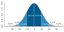
• Normal distribution (Gaussian distribution), for a single such quantity; the most commonly used continuous distribution

Exponential growth (e.g. prices, incomes, populations)[]

• Log-normal distribution, for a single such quantity whose log is normally distributed
• Pareto distribution, for a single such quantity whose log is exponentially distributed; the prototypical power law distribution

Uniformly distributed quantities[]

• Discrete uniform distribution, for a finite set of values (e.g. the outcome of a fair die)
• Continuous uniform distribution, for continuously distributed values

Bernoulli trials (yes/no events, with a given probability)[]

• Basic distributions:
  • Bernoulli distribution, for the outcome of a single Bernoulli trial (e.g. success/failure, yes/no)
  • Binomial distribution, for the number of "positive occurrences" (e.g. successes, yes votes, etc.) given a fixed total number of independent occurrences
  • Negative binomial distribution, for binomial-type observations but where the quantity of interest is the number of failures before a given number of successes occurs
  • Geometric distribution, for binomial-type observations but where the quantity of interest is the number of failures before the first success; a special case of the negative binomial distribution
• Related to sampling schemes over a finite population:
  • Hypergeometric distribution, for the number of "positive occurrences" (e.g. successes, yes votes, etc.) given a fixed number of total occurrences, using sampling without replacement
  • Beta-binomial distribution, for the number of "positive occurrences" (e.g. successes, yes votes, etc.) given a fixed number of total occurrences, sampling using a Pólya urn model (in some sense, the "opposite" of sampling without replacement)

Categorical outcomes (events with K possible outcomes)[]

• Categorical distribution, for a single categorical outcome (e.g. yes/no/maybe in a survey); a generalization of the Bernoulli distribution
• Multinomial distribution, for the number of each type of categorical outcome, given a fixed number of total outcomes; a generalization of the binomial distribution
• Multivariate hypergeometric distribution, similar to the multinomial distribution, but using sampling without replacement; a generalization of the hypergeometric distribution

Poisson process (events that occur independently with a given rate)[]

• Poisson distribution, for the number of occurrences of a Poisson-type event in a given period of time
• Exponential distribution, for the time before the next Poisson-type event occurs
• Gamma distribution, for the time before the next k Poisson-type events occur

Absolute values of vectors with normally distributed components[]

• Rayleigh distribution, for the distribution of vector magnitudes with Gaussian distributed orthogonal components. Rayleigh distributions are found in RF signals with Gaussian real and imaginary components.
• Rice distribution, a generalization of the Rayleigh distributions for where there is a stationary background signal component. Found in Rician fading of radio signals due to multipath propagation and in MR images with noise corruption on non-zero NMR signals.

Normally distributed quantities operated with sum of squares[]

• Chi-squared distribution, the distribution of a sum of squared standard normal variables; useful e.g. for inference regarding the sample variance of normally distributed samples (see chi-squared test)
• Student's t distribution, the distribution of the ratio of a standard normal variable and the square root of a scaled chi squared variable; useful for inference regarding the mean of normally distributed samples with unknown variance (see Student's t-test)
• F-distribution, the distribution of the ratio of two scaled chi squared variables; useful e.g. for inferences that involve comparing variances or involving R-squared (the squared correlation coefficient)

As conjugate prior distributions in Bayesian inference[]

• Beta distribution, for a single probability (real number between 0 and 1); conjugate to the Bernoulli distribution and binomial distribution
• Gamma distribution, for a non-negative scaling parameter; conjugate to the rate parameter of a Poisson distribution or exponential distribution, the precision (inverse variance) of a normal distribution, etc.
• Dirichlet distribution, for a vector of probabilities that must sum to 1; conjugate to the categorical distribution and multinomial distribution; generalization of the beta distribution
• Wishart distribution, for a symmetric non-negative definite matrix; conjugate to the inverse of the covariance matrix of a multivariate normal distribution; generalization of the gamma distribution^[30]

Some specialized applications of probability distributions[]

• The cache language models and other statistical language models used in natural language processing to assign probabilities to the occurrence of particular words and word sequences do so by means of probability distributions.
• In quantum mechanics, the probability density of finding the particle at a given point is proportional to the square of the magnitude of the particle's wavefunction at that point (see Born rule). Therefore, the probability distribution function of the position of a particle is described by ${\displaystyle P_{a\leq x\leq b}(t)=\int _{a}^{b}dx\,|\Psi (x,t)|^{2}}$, probability that the particle's position x will be in the interval a ≤ x ≤ b in dimension one, and a similar triple integral in dimension three. This is a key principle of quantum mechanics.^[31]
• Probabilistic load flow in power-flow study explains the uncertainties of input variables as probability distribution and provides the power flow calculation also in term of probability distribution.^[32]
• Prediction of natural phenomena occurrences based on previous frequency distributions such as tropical cyclones, hail, time in between events, etc.^[33]

See also[]

• Conditional probability distribution
• Joint probability distribution
• Quasiprobability distribution
• Empirical probability distribution
• Histogram
• Riemann–Stieltjes integral application to probability theory

Lists[]

• List of probability distributions
• List of statistical topics

References[]

Citations[]

Sources[]

External links[]

Wikimedia Commons has media related to Probability distribution.

• "Probability distribution", Encyclopedia of Mathematics, EMS Press, 2001 [1994]
• Field Guide to Continuous Probability Distributions, Gavin E. Crooks.