Romberg's method
In numerical analysis, Romberg's method (Romberg 1955) is used to estimate the definite integral

by applying Richardson extrapolation (Richardson 1911) repeatedly on the trapezium rule or the rectangle rule (midpoint rule). The estimates generate a triangular array. Romberg's method is a Newton–Cotes formula – it evaluates the integrand at equally spaced points. The integrand must have continuous derivatives, though fairly good results may be obtained if only a few derivatives exist. If it is possible to evaluate the integrand at unequally spaced points, then other methods such as Gaussian quadrature and Clenshaw–Curtis quadrature are generally more accurate.
The method is named after Werner Romberg (1909–2003), who published the method in 1955.
Method[]
Using

the method can be inductively defined by


or

where and . In big O notation, the error for R(n, m) is (Mysovskikh 2002):


The zeroeth extrapolation, R(n, 0), is equivalent to the trapezoidal rule with 2n + 1 points; the first extrapolation, R(n, 1), is equivalent to Simpson's rule with 2n + 1 points. The second extrapolation, R(n, 2), is equivalent to Boole's rule with 2n + 1 points. Further extrapolations differ from Newton-Cotes formulas. In particular further Romberg extrapolations expand on Boole's rule in very slight ways, modifying weights into ratios similar as in Boole's rule. In contrast, further Newton-Cotes methods produce increasingly differing weights, eventually leading to large positive and negative weights. This is indicative of how large degree interpolating polynomial Newton-Cotes methods fail to converge for many integrals, while Romberg integration is more stable.
When function evaluations are expensive, it may be preferable to replace the polynomial interpolation of Richardson with the rational interpolation proposed by Bulirsch & Stoer (1967).
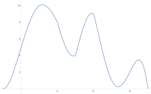
A geometric example[]
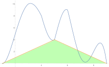
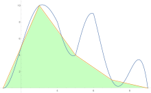
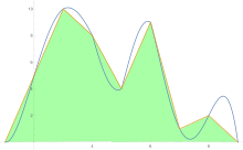
To estimate the area under a curve the trapezoid rule is applied first to one-piece, then two, then four, and so on.
After trapezoid rule estimates are obtained, Richardson extrapolation is applied.
- For the first iteration the two piece and one piece estimates are used in the formula (4 × (more accurate) − (less accurate))/3 The same formula is then used to compare the four piece and the two piece estimate, and likewise for the higher estimates
- For the second iteration the values of the first iteration are used in the formula (16(more accurate) − less accurate))/15
- The third iteration uses the next power of 4: (64 (more accurate) − less accurate))/63 on the values derived by the second iteration.
- The pattern is continued until there is one estimate.
| Number of pieces | Trapezoid estimates | First iteration | Second iteration | Third iteration |
|---|---|---|---|---|
| (4 MA − LA)/3* | (16 MA − LA)/15 | (64 MA − LA)/63 | ||
| 1 | 0 | (4×16 − 0)/3 = 21.333... | (16×34.667 − 21.333)/15 = 35.556... | (64×42.489 − 35.556)/63 = 42.599... |
| 2 | 16 | (4×30 − 16)/3 = 34.666... | (16×42 − 34.667)/15 = 42.489... | |
| 4 | 30 | (4×39 − 30)/3 = 42 | ||
| 8 | 39 |
- MA stands for more accurate, LA stands for less accurate
Example[]
As an example, the Gaussian function is integrated from 0 to 1, i.e. the error function erf(1) ≈ 0.842700792949715. The triangular array is calculated row by row and calculation is terminated if the two last entries in the last row differ less than 10−8.
 0.77174333
 0.82526296  0.84310283
 0.83836778  0.84273605  0.84271160
 0.84161922  0.84270304  0.84270083  0.84270066
 0.84243051  0.84270093  0.84270079  0.84270079  0.84270079
The result in the lower right corner of the triangular array is accurate to the digits shown. It is remarkable that this result is derived from the less accurate approximations obtained by the trapezium rule in the first column of the triangular array.
Implementation[]
Here is an example of a computer implementation of the Romberg method (in the C programming language).
#include <stdio.h>
#include <math.h>

void
dump_row(size_t i, double *R) {
   printf("R[%2zu] = ", i);
   for (size_t j = 0; j <= i; ++j){
      printf("%f ", R[j]);
   }
   printf("\n");
}

double
romberg(double (*f/* function to integrate */)(double), double /*lower limit*/ a, double /*upper limit*/ b, size_t max_steps, double /*desired accuracy*/ acc) {
   double R1[max_steps], R2[max_steps]; // buffers
   double *Rp = &R1[0], *Rc = &R2[0]; // Rp is previous row, Rc is current row
   double h = (b-a); //step size
   Rp[0] = (f(a) + f(b))*h*.5; // first trapezoidal step

   dump_row(0, Rp);

   for (size_t i = 1; i < max_steps; ++i) {
      h /= 2.;
      double c = 0;
      size_t ep = 1 << (i-1); //2^(n-1)
      for (size_t j = 1; j <= ep; ++j) {
         c += f(a+(2*j-1)*h);
      }
      Rc[0] = h*c + .5*Rp[0]; //R(i,0)

      for (size_t j = 1; j <= i; ++j) {
         double n_k = pow(4, j);
         Rc[j] = (n_k*Rc[j-1] - Rp[j-1])/(n_k-1); // compute R(i,j)
      }

      // Dump ith row of R, R[i,i] is the best estimate so far
      dump_row(i, Rc);

      if (i > 1 && fabs(Rp[i-1]-Rc[i]) < acc) {
         return Rc[i-1];
      }

      // swap Rn and Rc as we only need the last row
      double *rt = Rp;
      Rp = Rc;
      Rc = rt;
   }
   return Rp[max_steps-1]; // return our best guess
}
________________________________________________________
Here is an example of a computer implementation of the Romberg method (in the javascript programming language).
function auto_integrator_trap_romb_hnm(func,a,b,nmax,tol_ae,tol_rae)
// INPUTS
// func=integrand
// a= lower limit of integration
// b= upper limit of integration
// nmax = number of partitions, n=2^nmax
// tol_ae= maximum absolute approximate error acceptable (should be >=0)
// tol_rae=maximum absolute relative approximate error acceptable (should be >=0)
// OUTPUTS
// integ_value= estimated value of integral

{
	if (typeof a !== 'number')
		{
		  throw new TypeError('<a> must be a number');
		}
    if (typeof b !== 'number')
		{
		  throw new TypeError('<b> must be a number');
		}
    if ((!Number.isInteger(nmax)) || (nmax<1))
		{
		  throw new TypeError('<nmax> must be an integer greater than or equal to one.');
		}
	if ((typeof tol_ae !== 'number') || (tol_ae<0))
		{
		  throw new TypeError('<tole_ae> must be a number greater than or equal to zero');
		}
	if ((typeof tol_rae !== 'number') || (tol_rae<=0))
		{
		  throw new TypeError('<tole_ae> must be a number greater than or equal to zero');
		}

	var h=b-a
	// initialize matrix where the values of integral are stored

	var Romb = []; // rows
	for (var i = 0; i < nmax+1; i++)
	{
		Romb.push([]);
		for (var j = 0; j < nmax+1; j++)
		{
			Romb[i].push(math.bignumber(0));
		}
	}

	//calculating the value with 1-segment trapezoidal rule
	Romb[0][0]=0.5*h*(func(a)+func(b))
	var integ_val=Romb[0][0]

	for (var i=1; i<=nmax; i++)
	// updating the value with double the number of segments
	// by only using the values where they need to be calculated
	// See https://autarkaw.org/2009/02/28/an-efficient-formula-for-an-automatic-integrator-based-on-trapezoidal-rule/
	{
		h=0.5*h
		var integ=0
		for (var j=1; j<=2**i-1; j+=2)
		{
			var integ=integ+func(a+j*h)
		}

		Romb[i][0]=0.5*Romb[i-1][0]+integ*h
		// Using Romberg method to calculate next extrapolatable value
		// See https://young.physics.ucsc.edu/115/romberg.pdf
		for (k=1; k<=i; k++)
		{
			var addterm=Romb[i][k-1]-Romb[i-1][k-1]
			addterm=addterm/(4**k-1.0)
			Romb[i][k]=Romb[i][k-1]+addterm

			//Calculating absolute approximate error
			var Ea=math.abs(Romb[i][k]-Romb[i][k-1])

			//Calculating absolute relative approximate error
			var epsa=math.abs(Ea/Romb[i][k])*100.0

			//Assigning most recent value to the return variable
			integ_val=Romb[i][k]

			// returning the value if either tolerance is met
			if ((epsa<tol_rae) || (Ea<tol_ae))
			{
				return(integ_val)
			}
		}
	}
	// returning the last calculated value of integral whether tolerance is met or not
	return(integ_val)
}
References[]
- Richardson, L. F. (1911), "The Approximate Arithmetical Solution by Finite Differences of Physical Problems Involving Differential Equations, with an Application to the Stresses in a Masonry Dam", Philosophical Transactions of the Royal Society A, 210 (459–470): 307–357, doi:10.1098/rsta.1911.0009, JSTOR 90994
- Romberg, W. (1955), "Vereinfachte numerische Integration", Det Kongelige Norske Videnskabers Selskab Forhandlinger, Trondheim, 28 (7): 30–36
- Thacher Jr., Henry C. (July 1964), "Remark on Algorithm 60: Romberg integration", Communications of the ACM, 7 (7): 420–421, doi:10.1145/364520.364542
- Bauer, F.L.; Rutishauser, H.; Stiefel, E. (1963), Metropolis, N. C.; et al. (eds.), "New aspects in numerical quadrature", Experimental Arithmetic, high-speed computing and mathematics, Proceedings of Symposia in Applied Mathematics, AMS (15): 199–218
- Bulirsch, Roland; Stoer, Josef (1967), "Handbook Series Numerical Integration. Numerical quadrature by extrapolation", Numerische Mathematik, 9: 271–278, doi:10.1007/bf02162420
- Mysovskikh, I.P. (2002) [1994], "Romberg method", in Hazewinkel, Michiel (ed.), Encyclopedia of Mathematics, Springer-Verlag, ISBN 1-4020-0609-8
- Press, WH; Teukolsky, SA; Vetterling, WT; Flannery, BP (2007), "Section 4.3. Romberg Integration", Numerical Recipes: The Art of Scientific Computing (3rd ed.), New York: Cambridge University Press, ISBN 978-0-521-88068-8
External links[]
- ROMBINT – code for MATLAB (author: Martin Kacenak)
- Free online integration tool using Romberg, Fox–Romberg, Gauss–Legendre and other numerical methods
- SciPy implementation of Romberg's method
- Numerical integration (quadrature)