Sensitivity and specificity

Sensitivity and specificity - The left half of the image with the solid dots represents individuals who have the condition, while the right half of the image with the hollow dots represents individuals who do not have the condition. The circle represents all individuals who tested positive.

Sensitivity and specificity mathematically describe the accuracy of a test which reports the presence or absence of a condition, in comparison to a ‘Gold Standard’ or definition.

Sensitivity (True Positive Rate) refers to the proportion of those who have the condition (when judged by the ‘Gold Standard’) that received a positive result on this test.
Specificity (True Negative Rate) refers to the proportion of those who do not have the condition (when judged by the ‘Gold Standard’) that received a negative result on this test.

In a diagnostic test, sensitivity is a measure of how well a test can identify true positives and specificity is a measure of how well a test can identify true negatives. For all testing, both diagnostic and screening, there is usually a trade-off between sensitivity and specificity, such that higher sensitivities will mean lower specificities and vice versa.

If the goal of the test is to identify everyone who has a condition, the number of false negatives should be low, which requires high sensitivity. That is, people who have the condition should be highly likely to be identified as such by the test. This is especially important when the consequence of failing to treat the condition are serious and/or the treatment is very effective and has minimal side effects.

If the goal of the test is to accurately identify people who do not have the condition, the number of false positives should be very low, which requires a high specificity. That is, people who do not have the condition should be highly likely to be excluded by the test. This is especially important when people who are identified as having a condition may be subjected to more testing, expense, stigma, anxiety, etc.

Sensitivity and Specificity

The terms "sensitivity" and "specificity" were introduced by American biostatistician Jacob Yerushalmy in 1947.^[1]

Terminology and derivations
from a confusion matrix
condition positive (P) the number of real positive cases in the data condition negative (N) the number of real negative cases in the data true positive (TP) A test result that correctly indicates the presence of a condition or characteristic true negative (TN) A test result that correctly indicates the absence of a condition or characteristic false positive (FP) A test result which wrongly indicates that a particular condition or attribute is present false negative (FN) A test result which wrongly indicates that a particular condition or attribute is absent sensitivity, recall, hit rate, or true positive rate (TPR) $\mathrm {TPR} ={\frac {\mathrm {TP} }{\mathrm {P} }}={\frac {\mathrm {TP} }{\mathrm {TP} +\mathrm {FN} }}=1-\mathrm {FNR}$ specificity, selectivity or true negative rate (TNR) $\mathrm {TNR} ={\frac {\mathrm {TN} }{\mathrm {N} }}={\frac {\mathrm {TN} }{\mathrm {TN} +\mathrm {FP} }}=1-\mathrm {FPR}$ precision or positive predictive value (PPV) $\mathrm {PPV} ={\frac {\mathrm {TP} }{\mathrm {TP} +\mathrm {FP} }}=1-\mathrm {FDR}$ negative predictive value (NPV) $\mathrm {NPV} ={\frac {\mathrm {TN} }{\mathrm {TN} +\mathrm {FN} }}=1-\mathrm {FOR}$ miss rate or false negative rate (FNR) $\mathrm {FNR} ={\frac {\mathrm {FN} }{\mathrm {P} }}={\frac {\mathrm {FN} }{\mathrm {FN} +\mathrm {TP} }}=1-\mathrm {TPR}$ fall-out or false positive rate (FPR) $\mathrm {FPR} ={\frac {\mathrm {FP} }{\mathrm {N} }}={\frac {\mathrm {FP} }{\mathrm {FP} +\mathrm {TN} }}=1-\mathrm {TNR}$ false discovery rate (FDR) $\mathrm {FDR} ={\frac {\mathrm {FP} }{\mathrm {FP} +\mathrm {TP} }}=1-\mathrm {PPV}$ false omission rate (FOR) $\mathrm {FOR} ={\frac {\mathrm {FN} }{\mathrm {FN} +\mathrm {TN} }}=1-\mathrm {NPV}$ Positive likelihood ratio (LR+) $\mathrm {LR+} ={\frac {\mathrm {TPR} }{\mathrm {FPR} }}$ Negative likelihood ratio (LR-) $\mathrm {LR-} ={\frac {\mathrm {FNR} }{\mathrm {TNR} }}$ prevalence threshold (PT) $\mathrm {PT} ={\frac {{\sqrt {\mathrm {TPR} (-\mathrm {TNR} +1)}}+\mathrm {TNR} -1}{(\mathrm {TPR} +\mathrm {TNR} -1)}}={\frac {\sqrt {\mathrm {FPR} }}{{\sqrt {\mathrm {TPR} }}+{\sqrt {\mathrm {FPR} }}}}$ threat score (TS) or critical success index (CSI) $\mathrm {TS} ={\frac {\mathrm {TP} }{\mathrm {TP} +\mathrm {FN} +\mathrm {FP} }}$ Prevalence ${\frac {\mathrm {P} }{\mathrm {P} +\mathrm {N} }}$ accuracy (ACC) $\mathrm {ACC} ={\frac {\mathrm {TP} +\mathrm {TN} }{\mathrm {P} +\mathrm {N} }}={\frac {\mathrm {TP} +\mathrm {TN} }{\mathrm {TP} +\mathrm {TN} +\mathrm {FP} +\mathrm {FN} }}$ balanced accuracy (BA) $\mathrm {BA} ={\frac {TPR+TNR}{2}}$ F1 score is the harmonic mean of precision and sensitivity: $\mathrm {F} _{1}=2\times {\frac {\mathrm {PPV} \times \mathrm {TPR} }{\mathrm {PPV} +\mathrm {TPR} }}={\frac {2\mathrm {TP} }{2\mathrm {TP} +\mathrm {FP} +\mathrm {FN} }}$ phi coefficient (φ or r_φ) or Matthews correlation coefficient (MCC) $\mathrm {MCC} ={\frac {\mathrm {TP} \times \mathrm {TN} -\mathrm {FP} \times \mathrm {FN} }{\sqrt {(\mathrm {TP} +\mathrm {FP} )(\mathrm {TP} +\mathrm {FN} )(\mathrm {TN} +\mathrm {FP} )(\mathrm {TN} +\mathrm {FN} )}}}$ Fowlkes–Mallows index (FM) $\mathrm {FM} ={\sqrt {{\frac {TP}{TP+FP}}\times {\frac {TP}{TP+FN}}}}={\sqrt {PPV\times TPR}}$ informedness or bookmaker informedness (BM) $\mathrm {BM} =\mathrm {TPR} +\mathrm {TNR} -1$ markedness (MK) or deltaP (Δp) $\mathrm {MK} =\mathrm {PPV} +\mathrm {NPV} -1$ Diagnostic odds ratio (DOR) $\mathrm {DOR} ={\frac {\mathrm {LR+} }{\mathrm {LR-} }}$ Sources: Fawcett (2006),^[2] Piryonesi and El-Diraby (2020),^[3] Powers (2011),^[4] Ting (2011),^[5] CAWCR,^[6] D. Chicco & G. Jurman (2020, 2021),^[7]^[8] Tharwat (2018).^[9]

Application to screening study[]

Imagine a study evaluating a test that screens people for a disease. Each person taking the test either has or does not have the disease. The test outcome can be positive (classifying the person as having the disease) or negative (classifying the person as not having the disease). The test results for each subject may or may not match the subject's actual status. In that setting:

True positive: Sick people correctly identified as sick
False positive: Healthy people incorrectly identified as sick
True negative: Healthy people correctly identified as healthy
False negative: Sick people incorrectly identified as healthy

After getting the numbers of true positives, false positives, true negatives, and false negatives, the sensitivity and specificity for the test can be calculated. If it turns out that the sensitivity is high then any person who has the disease is likely to be classified as positive by the test. On the other hand, if the specificity is high, any person who does not have the disease is likely to be classified as negative by the test. An NIH web site has a discussion of how these ratios are calculated.^[10]

Definition[]

Sensitivity[]

Consider the example of a medical test for diagnosing a condition. Sensitivity refers to the test's ability to correctly detect ill patients who do have the condition.^[11] In the example of a medical test used to identify a condition, the sensitivity (sometimes also named the detection rate in a clinical setting) of the test is the proportion of people who test positive for the disease among those who have the disease. Mathematically, this can be expressed as:

{\begin{aligned}{\text{sensitivity}}&={\frac {\text{number of true positives}}{{\text{number of true positives}}+{\text{number of false negatives}}}}\\[8pt]&={\frac {\text{number of true positives}}{\text{total number of sick individuals in population}}}\\[8pt]&={\text{probability of a positive test given that the patient has the disease}}\end{aligned}}

A negative result in a test with high sensitivity is useful for ruling out disease.^[11] A high sensitivity test is reliable when its result is negative since it rarely misdiagnoses those who have the disease. A test with 100% sensitivity will recognize all patients with the disease by testing positive. A negative test result would definitively rule out presence of the disease in a patient. However, a positive result in a test with high sensitivity is not necessarily useful for ruling in disease. Suppose a 'bogus' test kit is designed to always give a positive reading. When used on diseased patients, all patients test positive, giving the test 100% sensitivity. However, sensitivity does not take into account false positives. The bogus test also returns positive on all healthy patients, giving it a false positive rate of 100%, rendering it useless for detecting or "ruling in" the disease.

The calculation of sensitivity does not take into account indeterminate test results. If a test cannot be repeated, indeterminate samples either should be excluded from the analysis (the number of exclusions should be stated when quoting sensitivity) or can be treated as false negatives (which gives the worst-case value for sensitivity and may therefore underestimate it).

Specificity[]

Consider the example of a medical test for diagnosing a disease. Specificity relates to the test's ability to correctly reject healthy patients without a condition. Specificity of a test is the proportion of those who truly do not have the condition who test negative for the condition. Mathematically, this can also be written as:

{\begin{aligned}{\text{specificity}}&={\frac {\text{number of true negatives}}{{\text{number of true negatives}}+{\text{number of false positives}}}}\\[8pt]&={\frac {\text{number of true negatives}}{\text{total number of well individuals in population}}}\\[8pt]&={\text{probability of a negative test given that the patient is well}}\end{aligned}}

A positive result in a test with high specificity is useful for ruling in disease. The test rarely gives positive results in healthy patients. A positive result signifies a high probability of the presence of disease.^[12] A test with 100% specificity will recognize all patients without the disease by testing negative, so a positive test result would definitely rule in the presence of the disease. However, a negative result from a test with high specificity is not necessarily useful for ruling out disease. For example, a test that always returns a negative test result will have a specificity of 100% because specificity does not consider false negatives. A test like that would return negative for patients with the disease, making it useless for ruling out the disease.

A test with a higher specificity has a lower type I error rate.

Graphical illustration[]

High sensitivity and low specificity
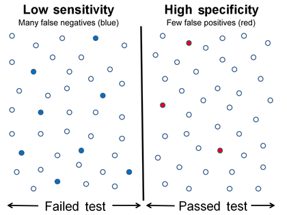
Low sensitivity and high specificity
A graphical illustration of sensitivity and specificity

The above graphical illustration is meant to show the relationship between sensitivity and specificity. The black, dotted line in the center of the graph is where the sensitivity and specificity are the same. As one moves to the left of the black, dotted line the sensitivity increases, reaching its maximum value of 100% at line A, and the specificity decreases. The sensitivity at line A is 100% because at that point there are zero false negatives, meaning that all the negative test results are true negatives. When moving to the right, the opposite applies, the specificity increases until it reaches the B line and becomes 100% and the sensitivity decreases. The specificity at line B is 100% because the number of false positives is zero at that line, meaning all the positive test results are true positives.

The middle solid line in both figures that show the level of sensitivity and specificity is the test cutoff point. Moving this line resulting in the trade-off between the level of sensitivity and specificity as previously described. The left-hand side of this line contains the data points that have the condition (the blue dots indicate the false negatives). The right-hand side of the line shows the data points that do not have the condition (red dots indicate false positives). The total number of data points is 80. 40 of them have a medical condition and are on the left side. The rest is on the right side and do not have the medical condition.

For the figure that shows high sensitivity and low specificity, the number of false negatives is 3, and the number of data point that has the medical condition is 40, so the sensitivity is (40 − 3) / (37 + 3) = 92.5%. The number of false positives is 9, so the specificity is (40 − 9) / 40 = 77.5%. Similarly, the number of false negatives in another figure is 8, and the number of data point that has the medical condition is 40, so the sensitivity is (40 − 8) / (37 + 3) = 80%. The number of false positives is 3, so the specificity is (40 − 3) / 40 = 92.5%.

A test result with 100 percent sensitivity.
A test result with 100 percent specificity.

The red dot indicates the patient with the medical condition. The red background indicates the area where the test predicts the data point to be positive. The true positive in this figure is 6, and false negatives of 0 (because all positive condition is correctly predicted as positive). Therefore the sensitivity is 100% (from 6 / (6 + 0)). This situation is also illustrated in the previous figure where the dotted line is at position A (the left-hand side is predicted as negative by the model, the right-hand side is predicted as positive by the model). When the dotted line, test cut-off line, is at position A, the test correctly predicts all the population of the true positive class, but it will fail to correctly identify the data point from the true negative class.

Similar to the previously explained figure, the red dot indicates the patient with the medical condition. However, in this case, the green background indicates that the test predicts that all patients are free of the medical condition. The number of data point that is true negative is then 26, and the number of false positives is 0. This result in 100% specificity (from 26 / (26 + 0)). Therefore, sensitivity or specificity alone cannot be used to measure the performance of the test.

Medical usage[]

In medical diagnosis, test sensitivity is the ability of a test to correctly identify those with the disease (true positive rate), whereas test specificity is the ability of the test to correctly identify those without the disease (true negative rate). If 100 patients known to have a disease were tested, and 43 test positive, then the test has 43% sensitivity. If 100 with no disease are tested and 96 return a completely negative result, then the test has 96% specificity. Sensitivity and specificity are prevalence-independent test characteristics, as their values are intrinsic to the test and do not depend on the disease prevalence in the population of interest.^[13] Positive and negative predictive values, but not sensitivity or specificity, are values influenced by the prevalence of disease in the population that is being tested. These concepts are illustrated graphically in this applet Bayesian clinical diagnostic model which show the positive and negative predictive values as a function of the prevalence, sensitivity and specificity.

Misconceptions[]

It is often claimed that a highly specific test is effective at ruling in a disease when positive, while a highly sensitive test is deemed effective at ruling out a disease when negative.^[14]^[15] This has led to the widely used mnemonics SPPIN and SNNOUT, according to which a highly specific test, when positive, rules in disease (SP-P-IN), and a highly 'sensitive' test, when negative rules out disease (SN-N-OUT). Both rules of thumb are, however, inferentially misleading, as the diagnostic power of any test is determined by both its sensitivity and its specificity.^[16]^[17]^[18]

The tradeoff between specificity and sensitivity is explored in ROC analysis as a trade off between TPR and FPR (that is, recall and fallout).^[19] Giving them equal weight optimizes informedness = specificity + sensitivity − 1 = TPR − FPR, the magnitude of which gives the probability of an informed decision between the two classes (> 0 represents appropriate use of information, 0 represents chance-level performance, < 0 represents perverse use of information).^[20]

Sensitivity index[]

The sensitivity index or d' (pronounced 'dee-prime') is a statistic used in signal detection theory. It provides the separation between the means of the signal and the noise distributions, compared against the standard deviation of the noise distribution. For normally distributed signal and noise with mean and standard deviations $\mu _{S}$ and $\sigma _{S}$ , and $\mu _{N}$ and $\sigma _{N}$ , respectively, d' is defined as:

d'={\frac {\mu _{S}-\mu _{N}}{\sqrt {{\frac {1}{2}}\left(\sigma _{S}^{2}+\sigma _{N}^{2}\right)}}}

^[21]

An estimate of d' can be also found from measurements of the hit rate and false-alarm rate. It is calculated as:

d' = Z(hit rate) − Z(false alarm rate),^[22]

where function Z(p), p ∈ [0, 1], is the inverse of the cumulative Gaussian distribution.

d' is a dimensionless statistic. A higher d' indicates that the signal can be more readily detected.

Confusion matrix[]

The relationship between sensitivity, specificity, and similar terms can be understood using the following table. Consider a group with P positive instances and N negative instances of some condition. The four outcomes can be formulated in a 2×2 contingency table or confusion matrix, as well as derivations of several metrics using the four outcomes, as follows:

		Predicted condition		^Sources:^[23]^[24]^[25]^[26]^[27]^[28]^[29]^[30] ^view talk
	Total population = P + N	Positive (PP)	Negative (PN)	Informedness, bookmaker informedness (BM) = TPR + TNR − 1	Prevalence threshold (PT) = √TPR × FPR − FPR/TPR − FPR
Actual condition	Positive (P)	True positive (TP), hit	False negative (FN), type II error, miss, underestimation	True positive rate (TPR), recall, sensitivity (SEN), probability of detection, hit rate, power = TP/P = 1 − FNR	False negative rate (FNR), miss rate = FN/P = 1 − TPR
Actual condition	Negative (N)	False positive (FP), type I error, false alarm, overestimation	True negative (TN), correct rejection	False positive rate (FPR), probability of false alarm, fall-out = FP/N = 1 − TNR	True negative rate (TNR), specificity (SPC), selectivity = TN/N = 1 − FPR
	Prevalence = P/P + N	Positive predictive value (PPV), precision = TP/PP = 1 − FDR	False omission rate (FOR) = FN/PN = 1 − NPV	Positive likelihood ratio (LR+) = TPR/FPR	Negative likelihood ratio (LR−) = FNR/TNR
	Accuracy (ACC) = TP + TN/P + N	False discovery rate (FDR) = FP/PP = 1 − PPV	Negative predictive value (NPV) = TN/PN = 1 − FOR	Markedness (MK), deltaP (Δp) = PPV + NPV − 1	Diagnostic odds ratio (DOR) = LR+/LR−
	Balanced accuracy (BA) = TPR + TNR/2	F₁ score = 2 PPV × TPR/PPV + TPR = 2 TP/2 TP + FP + FN	Fowlkes–Mallows index (FM) = √PPV×TPR	Matthews correlation coefficient (MCC) = √TPR×TNR×PPV×NPV − √FNR×FPR×FOR×FDR	Threat score (TS), critical success index (CSI), Jaccard index = TP/TP + FN + FP

A worked example: A diagnostic test with sensitivity 67% and specificity 91% is applied to 2030 people to look for a disorder with a population prevalence of 1.48%

		Fecal occult blood screen test outcome		^view
	Total population (pop.) = 2030	Test outcome positive	Test outcome negative	Accuracy (ACC) = (TP + TN) / pop. = (20 + 1820) / 2030 ≈ 90.64%	F₁ score = 2 × precision × recall/precision + recall ≈ 0.174
Patients with bowel cancer (as confirmed on endoscopy)	Actual condition positive	True positive (TP) = 20 (2030 × 1.48% × 67%)	False negative (FN) = 10 (2030 × 1.48% × (100% − 67%))	True positive rate (TPR), recall, sensitivity = TP / (TP + FN) = 20 / (20 + 10) ≈ 66.7%	False negative rate (FNR), miss rate = FN / (TP + FN) = 10 / (20 + 10) ≈ 33.3%
Patients with bowel cancer (as confirmed on endoscopy)	Actual condition negative	False positive (FP) = 180 (2030 × (100% − 1.48%) × (100% − 91%))	True negative (TN) = 1820 (2030 × (100% − 1.48%) × 91%)	False positive rate (FPR), fall-out, probability of false alarm = FP / (FP + TN) = 180 / (180 + 1820) = 9.0%	Specificity, selectivity, true negative rate (TNR) = TN / (FP + TN) = 1820 / (180 + 1820) = 91%
	Prevalence = (TP + FN) / pop. = (20 + 10) / 2030 ≈ 1.48%	Positive predictive value (PPV), precision = TP / (TP + FP) = 20 / (20 + 180) = 10%	False omission rate (FOR) = FN / (FN + TN) = 10 / (10 + 1820) ≈ 0.55%	Positive likelihood ratio (LR+) = TPR/FPR = (20 / 30) / (180 / 2000) ≈ 7.41	Negative likelihood ratio (LR−) = FNR/TNR = (10 / 30) / (1820 / 2000) ≈ 0.366
		False discovery rate (FDR) = FP / (TP + FP) = 180 / (20 + 180) = 90.0%	Negative predictive value (NPV) = TN / (FN + TN) = 1820 / (10 + 1820) ≈ 99.45%	Diagnostic odds ratio (DOR) = LR+/LR− ≈ 20.2

Related calculations

False positive rate (α) = type I error = 1 − specificity = FP / (FP + TN) = 180 / (180 + 1820) = 9%
False negative rate (β) = type II error = 1 − sensitivity = FN / (TP + FN) = 10 / (20 + 10) ≈ 33%
Power = sensitivity = 1 − β
Positive likelihood ratio = sensitivity / (1 − specificity) ≈ 0.67 / (1 − 0.91) ≈ 7.4
Negative likelihood ratio = (1 − sensitivity) / specificity ≈ (1 − 0.67) / 0.91 ≈ 0.37
Prevalence threshold = $PT={\frac {{\sqrt {TPR(-TNR+1)}}+TNR-1}{(TPR+TNR-1)}}$ ≈ 0.2686 ≈ 26.9%

This hypothetical screening test (fecal occult blood test) correctly identified two-thirds (66.7%) of patients with colorectal cancer.^[a] Unfortunately, factoring in prevalence rates reveals that this hypothetical test has a high false positive rate, and it does not reliably identify colorectal cancer in the overall population of asymptomatic people (PPV = 10%).

On the other hand, this hypothetical test demonstrates very accurate detection of cancer-free individuals (NPV ≈ 99.5%). Therefore, when used for routine colorectal cancer screening with asymptomatic adults, a negative result supplies important data for the patient and doctor, such as ruling out cancer as the cause of gastrointestinal symptoms or reassuring patients worried about developing colorectal cancer.

Estimation of errors in quoted sensitivity or specificity[]

Sensitivity and specificity values alone may be highly misleading. The 'worst-case' sensitivity or specificity must be calculated in order to avoid reliance on experiments with few results. For example, a particular test may easily show 100% sensitivity if tested against the gold standard four times, but a single additional test against the gold standard that gave a poor result would imply a sensitivity of only 80%. A common way to do this is to state the binomial proportion confidence interval, often calculated using a Wilson score interval.

Confidence intervals for sensitivity and specificity can be calculated, giving the range of values within which the correct value lies at a given confidence level (e.g., 95%).^[33]

Terminology in information retrieval[]

In information retrieval, the positive predictive value is called precision, and sensitivity is called recall. Unlike the Specificity vs Sensitivity tradeoff, these measures are both independent of the number of true negatives, which is generally unknown and much larger than the actual numbers of relevant and retrieved documents. This assumption of very large numbers of true negatives versus positives is rare in other applications.^[20]

The F-score can be used as a single measure of performance of the test for the positive class. The F-score is the harmonic mean of precision and recall:

F=2\times {\frac {{\text{precision}}\times {\text{recall}}}{{\text{precision}}+{\text{recall}}}}

In the traditional language of statistical hypothesis testing, the sensitivity of a test is called the statistical power of the test, although the word power in that context has a more general usage that is not applicable in the present context. A sensitive test will have fewer Type II errors.

Notes[]

^ There are advantages and disadvantages for all medical screening tests. Clinical practice guidelines, such as those for colorectal cancer screening, describe these risks and benefits.^[31]^[32]

References[]

^ Yerushalmy J (1947). "Statistical problems in assessing methods of medical diagnosis with special reference to x-ray techniques". Public Health Reports. 62 (2): 1432–39. doi:10.2307/4586294. JSTOR 4586294. PMID 20340527.
^ Fawcett, Tom (2006). "An Introduction to ROC Analysis" (PDF). Pattern Recognition Letters. 27 (8): 861–874. doi:10.1016/j.patrec.2005.10.010.
^ Piryonesi S. Madeh; El-Diraby Tamer E. (2020-03-01). "Data Analytics in Asset Management: Cost-Effective Prediction of the Pavement Condition Index". Journal of Infrastructure Systems. 26 (1): 04019036. doi:10.1061/(ASCE)IS.1943-555X.0000512.
^ Powers, David M. W. (2011). "Evaluation: From Precision, Recall and F-Measure to ROC, Informedness, Markedness & Correlation". Journal of Machine Learning Technologies. 2 (1): 37–63.
^ Ting, Kai Ming (2011). Sammut, Claude; Webb, Geoffrey I. (eds.). Encyclopedia of machine learning. Springer. doi:10.1007/978-0-387-30164-8. ISBN 978-0-387-30164-8.
^ Brooks, Harold; Brown, Barb; Ebert, Beth; Ferro, Chris; Jolliffe, Ian; Koh, Tieh-Yong; Roebber, Paul; Stephenson, David (2015-01-26). "WWRP/WGNE Joint Working Group on Forecast Verification Research". Collaboration for Australian Weather and Climate Research. World Meteorological Organisation. Retrieved 2019-07-17.
^ Chicco D.; Jurman G. (January 2020). "The advantages of the Matthews correlation coefficient (MCC) over F1 score and accuracy in binary classification evaluation". BMC Genomics. 21 (1): 6-1–6-13. doi:10.1186/s12864-019-6413-7. PMC 6941312. PMID 31898477.
^ Chicco D.; Toetsch N.; Jurman G. (February 2021). "The Matthews correlation coefficient (MCC) is more reliable than balanced accuracy, bookmaker informedness, and markedness in two-class confusion matrix evaluation". BioData Mining. 14 (13): 1-22. doi:10.1186/s13040-021-00244-z. PMC 7863449. PMID 33541410.
^ Tharwat A. (August 2018). "Classification assessment methods". Applied Computing and Informatics. doi:10.1016/j.aci.2018.08.003.
^ Parikh, Rajul; Mathai, Annie; Parikh, Shefali; Chandra Sekhar, G; Thomas, Ravi (2008). "Understanding and using sensitivity, specificity and predictive values". Indian Journal of Ophthalmology. 56 (1): 45–50. doi:10.4103/0301-4738.37595. PMC 2636062. PMID 18158403.
^ ^a ^b Altman DG, Bland JM (June 1994). "Diagnostic tests. 1: Sensitivity and specificity". BMJ. 308 (6943): 1552. doi:10.1136/bmj.308.6943.1552. PMC 2540489. PMID 8019315.
^ "SpPins and SnNouts". Centre for Evidence Based Medicine (CEBM). Retrieved 26 December 2013.
^ Mangrulkar R. "Diagnostic Reasoning I and II". Retrieved 24 January 2012.
^ "Evidence-Based Diagnosis". Michigan State University. Archived from the original on 2013-07-06. Retrieved 2013-08-23.
^ "Sensitivity and Specificity". Emory University Medical School Evidence Based Medicine course.
^ Baron JA (Apr–Jun 1994). "Too bad it isn't true". Medical Decision Making. 14 (2): 107. doi:10.1177/0272989X9401400202. PMID 8028462. S2CID 44505648.
^ Boyko EJ (Apr–Jun 1994). "Ruling out or ruling in disease with the most sensitive or specific diagnostic test: short cut or wrong turn?". Medical Decision Making. 14 (2): 175–9. doi:10.1177/0272989X9401400210. PMID 8028470. S2CID 31400167.
^ Pewsner D, Battaglia M, Minder C, Marx A, Bucher HC, Egger M (July 2004). "Ruling a diagnosis in or out with "SpPIn" and "SnNOut": a note of caution". BMJ. 329 (7459): 209–13. doi:10.1136/bmj.329.7459.209. PMC 487735. PMID 15271832.
^ Fawcett, Tom (2006). "An Introduction to ROC Analysis". Pattern Recognition Letters. 27 (8): 861–874. Bibcode:2006PaReL..27..861F. doi:10.1016/j.patrec.2005.10.010.
^ ^a ^b Powers, David M. W. (2011). "Evaluation: From Precision, Recall and F-Measure to ROC, Informedness, Markedness & Correlation". Journal of Machine Learning Technologies. 2 (1): 37–63.
^ Gale SD, Perkel DJ (January 2010). "A basal ganglia pathway drives selective auditory responses in songbird dopaminergic neurons via disinhibition". The Journal of Neuroscience. 30 (3): 1027–37. doi:10.1523/JNEUROSCI.3585-09.2010. PMC 2824341. PMID 20089911.
^ Macmillan NA, Creelman CD (15 September 2004). Detection Theory: A User's Guide. Psychology Press. p. 7. ISBN 978-1-4106-1114-7.
^ Fawcett, Tom (2006). "An Introduction to ROC Analysis" (PDF). Pattern Recognition Letters. 27 (8): 861–874. doi:10.1016/j.patrec.2005.10.010.
^ Piryonesi S. Madeh; El-Diraby Tamer E. (2020-03-01). "Data Analytics in Asset Management: Cost-Effective Prediction of the Pavement Condition Index". Journal of Infrastructure Systems. 26 (1): 04019036. doi:10.1061/(ASCE)IS.1943-555X.0000512.
^ Powers, David M. W. (2011). "Evaluation: From Precision, Recall and F-Measure to ROC, Informedness, Markedness & Correlation". Journal of Machine Learning Technologies. 2 (1): 37–63.
^ Ting, Kai Ming (2011). Sammut, Claude; Webb, Geoffrey I. (eds.). Encyclopedia of machine learning. Springer. doi:10.1007/978-0-387-30164-8. ISBN 978-0-387-30164-8.
^ Brooks, Harold; Brown, Barb; Ebert, Beth; Ferro, Chris; Jolliffe, Ian; Koh, Tieh-Yong; Roebber, Paul; Stephenson, David (2015-01-26). "WWRP/WGNE Joint Working Group on Forecast Verification Research". Collaboration for Australian Weather and Climate Research. World Meteorological Organisation. Retrieved 2019-07-17.
^ Chicco D, Jurman G (January 2020). "The advantages of the Matthews correlation coefficient (MCC) over F1 score and accuracy in binary classification evaluation". BMC Genomics. 21 (1): 6-1–6-13. doi:10.1186/s12864-019-6413-7. PMC 6941312. PMID 31898477.
^ Chicco D, Toetsch N, Jurman G (February 2021). "The Matthews correlation coefficient (MCC) is more reliable than balanced accuracy, bookmaker informedness, and markedness in two-class confusion matrix evaluation". BioData Mining. 14 (13): 1-22. doi:10.1186/s13040-021-00244-z. PMC 7863449. PMID 33541410.
^ Tharwat A. (August 2018). "Classification assessment methods". Applied Computing and Informatics. doi:10.1016/j.aci.2018.08.003.
^ Lin, Jennifer S.; Piper, Margaret A.; Perdue, Leslie A.; Rutter, Carolyn M.; Webber, Elizabeth M.; O’Connor, Elizabeth; Smith, Ning; Whitlock, Evelyn P. (21 June 2016). "Screening for Colorectal Cancer". JAMA. 315 (23): 2576–2594. doi:10.1001/jama.2016.3332. ISSN 0098-7484.
^ Bénard, Florence; Barkun, Alan N.; Martel, Myriam; Renteln, Daniel von (7 January 2018). "Systematic review of colorectal cancer screening guidelines for average-risk adults: Summarizing the current global recommendations". World Journal of Gastroenterology. 24 (1): 124–138. doi:10.3748/wjg.v24.i1.124. PMC 5757117. PMID 29358889.
^ "Diagnostic test online calculator calculates sensitivity, specificity, likelihood ratios and predictive values from a 2x2 table – calculator of confidence intervals for predictive parameters". medcalc.org.

External links[]

[33] There are advantages and disadvantages for all medical screening tests. Clinical practice guidelines, such as those for colorectal cancer screening, describe these risks and benefits.^[31]^[32]

[1] Yerushalmy J (1947). "Statistical problems in assessing methods of medical diagnosis with special reference to x-ray techniques". Public Health Reports. 62 (2): 1432–39. doi:10.2307/4586294. JSTOR 4586294. PMID 20340527.

[2] Fawcett, Tom (2006). "An Introduction to ROC Analysis" (PDF). Pattern Recognition Letters. 27 (8): 861–874. doi:10.1016/j.patrec.2005.10.010.

[3] Piryonesi S. Madeh; El-Diraby Tamer E. (2020-03-01). "Data Analytics in Asset Management: Cost-Effective Prediction of the Pavement Condition Index". Journal of Infrastructure Systems. 26 (1): 04019036. doi:10.1061/(ASCE)IS.1943-555X.0000512.

[4] Powers, David M. W. (2011). "Evaluation: From Precision, Recall and F-Measure to ROC, Informedness, Markedness & Correlation". Journal of Machine Learning Technologies. 2 (1): 37–63.

[5] Ting, Kai Ming (2011). Sammut, Claude; Webb, Geoffrey I. (eds.). Encyclopedia of machine learning. Springer. doi:10.1007/978-0-387-30164-8. ISBN 978-0-387-30164-8.

[6] Brooks, Harold; Brown, Barb; Ebert, Beth; Ferro, Chris; Jolliffe, Ian; Koh, Tieh-Yong; Roebber, Paul; Stephenson, David (2015-01-26). "WWRP/WGNE Joint Working Group on Forecast Verification Research". Collaboration for Australian Weather and Climate Research. World Meteorological Organisation. Retrieved 2019-07-17.

[7] Chicco D.; Jurman G. (January 2020). "The advantages of the Matthews correlation coefficient (MCC) over F1 score and accuracy in binary classification evaluation". BMC Genomics. 21 (1): 6-1–6-13. doi:10.1186/s12864-019-6413-7. PMC 6941312. PMID 31898477.

[8] Chicco D.; Toetsch N.; Jurman G. (February 2021). "The Matthews correlation coefficient (MCC) is more reliable than balanced accuracy, bookmaker informedness, and markedness in two-class confusion matrix evaluation". BioData Mining. 14 (13): 1-22. doi:10.1186/s13040-021-00244-z. PMC 7863449. PMID 33541410.

[9] Tharwat A. (August 2018). "Classification assessment methods". Applied Computing and Informatics. doi:10.1016/j.aci.2018.08.003.

[10] Parikh, Rajul; Mathai, Annie; Parikh, Shefali; Chandra Sekhar, G; Thomas, Ravi (2008). "Understanding and using sensitivity, specificity and predictive values". Indian Journal of Ophthalmology. 56 (1): 45–50. doi:10.4103/0301-4738.37595. PMC 2636062. PMID 18158403.

[BMJ-11] Altman DG, Bland JM (June 1994). "Diagnostic tests. 1: Sensitivity and specificity". BMJ. 308 (6943): 1552. doi:10.1136/bmj.308.6943.1552. PMC 2540489. PMID 8019315.

[cebm-12] "SpPins and SnNouts". Centre for Evidence Based Medicine (CEBM). Retrieved 26 December 2013.

[13] Mangrulkar R. "Diagnostic Reasoning I and II". Retrieved 24 January 2012.

[14] "Evidence-Based Diagnosis". Michigan State University. Archived from the original on 2013-07-06. Retrieved 2013-08-23.

[15] "Sensitivity and Specificity". Emory University Medical School Evidence Based Medicine course.

[pmid8028462-16] Baron JA (Apr–Jun 1994). "Too bad it isn't true". Medical Decision Making. 14 (2): 107. doi:10.1177/0272989X9401400202. PMID 8028462. S2CID 44505648.

[pmid8028470-17] Boyko EJ (Apr–Jun 1994). "Ruling out or ruling in disease with the most sensitive or specific diagnostic test: short cut or wrong turn?". Medical Decision Making. 14 (2): 175–9. doi:10.1177/0272989X9401400210. PMID 8028470. S2CID 31400167.

[pmid15271832-18] Pewsner D, Battaglia M, Minder C, Marx A, Bucher HC, Egger M (July 2004). "Ruling a diagnosis in or out with "SpPIn" and "SnNOut": a note of caution". BMJ. 329 (7459): 209–13. doi:10.1136/bmj.329.7459.209. PMC 487735. PMID 15271832.

[Fawcett2006-19] Fawcett, Tom (2006). "An Introduction to ROC Analysis". Pattern Recognition Letters. 27 (8): 861–874. Bibcode:2006PaReL..27..861F. doi:10.1016/j.patrec.2005.10.010.

[Powers2011-20] Powers, David M. W. (2011). "Evaluation: From Precision, Recall and F-Measure to ROC, Informedness, Markedness & Correlation". Journal of Machine Learning Technologies. 2 (1): 37–63.

[pmid20089911-21] Gale SD, Perkel DJ (January 2010). "A basal ganglia pathway drives selective auditory responses in songbird dopaminergic neurons via disinhibition". The Journal of Neuroscience. 30 (3): 1027–37. doi:10.1523/JNEUROSCI.3585-09.2010. PMC 2824341. PMID 20089911.

[MacmillanCreelman2004-22] Macmillan NA, Creelman CD (15 September 2004). Detection Theory: A User's Guide. Psychology Press. p. 7. ISBN 978-1-4106-1114-7.

[23] Fawcett, Tom (2006). "An Introduction to ROC Analysis" (PDF). Pattern Recognition Letters. 27 (8): 861–874. doi:10.1016/j.patrec.2005.10.010.

[24] Piryonesi S. Madeh; El-Diraby Tamer E. (2020-03-01). "Data Analytics in Asset Management: Cost-Effective Prediction of the Pavement Condition Index". Journal of Infrastructure Systems. 26 (1): 04019036. doi:10.1061/(ASCE)IS.1943-555X.0000512.

[25] Powers, David M. W. (2011). "Evaluation: From Precision, Recall and F-Measure to ROC, Informedness, Markedness & Correlation". Journal of Machine Learning Technologies. 2 (1): 37–63.

[26] Ting, Kai Ming (2011). Sammut, Claude; Webb, Geoffrey I. (eds.). Encyclopedia of machine learning. Springer. doi:10.1007/978-0-387-30164-8. ISBN 978-0-387-30164-8.

[27] Brooks, Harold; Brown, Barb; Ebert, Beth; Ferro, Chris; Jolliffe, Ian; Koh, Tieh-Yong; Roebber, Paul; Stephenson, David (2015-01-26). "WWRP/WGNE Joint Working Group on Forecast Verification Research". Collaboration for Australian Weather and Climate Research. World Meteorological Organisation. Retrieved 2019-07-17.

[28] Chicco D, Jurman G (January 2020). "The advantages of the Matthews correlation coefficient (MCC) over F1 score and accuracy in binary classification evaluation". BMC Genomics. 21 (1): 6-1–6-13. doi:10.1186/s12864-019-6413-7. PMC 6941312. PMID 31898477.

[29] Chicco D, Toetsch N, Jurman G (February 2021). "The Matthews correlation coefficient (MCC) is more reliable than balanced accuracy, bookmaker informedness, and markedness in two-class confusion matrix evaluation". BioData Mining. 14 (13): 1-22. doi:10.1186/s13040-021-00244-z. PMC 7863449. PMID 33541410.

[30] Tharwat A. (August 2018). "Classification assessment methods". Applied Computing and Informatics. doi:10.1016/j.aci.2018.08.003.

[31] Lin, Jennifer S.; Piper, Margaret A.; Perdue, Leslie A.; Rutter, Carolyn M.; Webber, Elizabeth M.; O’Connor, Elizabeth; Smith, Ning; Whitlock, Evelyn P. (21 June 2016). "Screening for Colorectal Cancer". JAMA. 315 (23): 2576–2594. doi:10.1001/jama.2016.3332. ISSN 0098-7484.

[32] Bénard, Florence; Barkun, Alan N.; Martel, Myriam; Renteln, Daniel von (7 January 2018). "Systematic review of colorectal cancer screening guidelines for average-risk adults: Summarizing the current global recommendations". World Journal of Gastroenterology. 24 (1): 124–138. doi:10.3748/wjg.v24.i1.124. PMC 5757117. PMID 29358889.

[34] "Diagnostic test online calculator calculates sensitivity, specificity, likelihood ratios and predictive values from a 2x2 table – calculator of confidence intervals for predictive parameters". medcalc.org.

[1]

[2]

[3]

[4]

[5]

[6]

[7]

[8]

[9]

[10]

[11]

[12]

[13]

[14]

[15]

[16]

[17]

[18]

[19]

[20]

[21]

[22]

[23]

[24]

[25]

[26]

[27]

[28]

[29]

[30]

[a]

[33]

[31]

[32]