Smith chart

The Smith chart, invented by Phillip H. Smith (1905–1987)^[1][2] and independently^[3] by Mizuhashi Tosaku,^[4] is a graphical calculator or nomogram designed for electrical and electronics engineers specializing in radio frequency (RF) engineering to assist in solving problems with transmission lines and matching circuits.^[5][6] The Smith chart can be used to simultaneously display multiple parameters including impedances, admittances, reflection coefficients, ${\displaystyle S_{nn}\,}$ scattering parameters, noise figure circles, constant gain contours and regions for unconditional stability, including mechanical vibrations analysis.^{[7][8]: 93–103} The Smith chart is most frequently used at or within the unity radius region. However, the remainder is still mathematically relevant, being used, for example, in oscillator design and stability analysis.^{[8]: 98–101} While the use of paper Smith charts for solving the complex mathematics involved in matching problems has been largely replaced by software based methods, the Smith chart is still a very useful method of showing ^[9] how RF parameters behave at one or more frequencies, an alternative to using tabular information. Thus most RF circuit analysis software includes a Smith chart option for the display of results and all but the simplest impedance measuring instruments can plot measured results on a Smith chart display.^[10]

An impedance Smith chart (with no data plotted)

Overview[]

A network analyzer (HP 8720A) showing a Smith chart.

The Smith chart is plotted on the complex reflection coefficient plane in two dimensions and is scaled in normalised impedance (the most common), normalised admittance or both, using different colours to distinguish between them. These are often known as the Z, Y and YZ Smith charts respectively.^[8]: 97 Normalised scaling allows the Smith chart to be used for problems involving any characteristic or system impedance which is represented by the center point of the chart. The most commonly used normalization impedance is 50 ohms. Once an answer is obtained through the graphical constructions described below, it is straightforward to convert between normalised impedance (or normalised admittance) and the corresponding unnormalized value by multiplying by the characteristic impedance (admittance). Reflection coefficients can be read directly from the chart as they are unitless parameters.

The Smith chart has a scale around its circumference or periphery which is graduated in wavelengths and degrees. The wavelengths scale is used in distributed component problems and represents the distance measured along the transmission line connected between the generator or source and the load to the point under consideration. The degrees scale represents the angle of the voltage reflection coefficient at that point. The Smith chart may also be used for lumped-element matching and analysis problems.

Use of the Smith chart and the interpretation of the results obtained using it requires a good understanding of AC circuit theory and transmission-line theory, both of which are prerequisites for RF engineers.

As impedances and admittances change with frequency, problems using the Smith chart can only be solved manually using one frequency at a time, the result being represented by a point. This is often adequate for narrow band applications (typically up to about 5% to 10% bandwidth) but for wider bandwidths it is usually necessary to apply Smith chart techniques at more than one frequency across the operating frequency band. Provided the frequencies are sufficiently close, the resulting Smith chart points may be joined by straight lines to create a locus.

A locus of points on a Smith chart covering a range of frequencies can be used to visually represent:

• how capacitive or how inductive a load is across the frequency range
• how difficult matching is likely to be at various frequencies
• how well matched a particular component is.

The accuracy of the Smith chart is reduced for problems involving a large locus of impedances or admittances, although the scaling can be magnified for individual areas to accommodate these.

Mathematical basis[]

Most basic use of an impedance Smith chart. A wave travels down a transmission line of characteristic impedance Z₀, terminated at a load with impedance Z_L and normalised impedance z=Z_L/Z₀. There is a signal reflection with coefficient Γ. Each point on the Smith chart simultaneously represents both a value of z (bottom left), and the corresponding value of Γ (bottom right), related by z=(1 + Γ)/(1 − Γ).

Actual and normalised impedance and admittance[]

A transmission line with a characteristic impedance of ${\displaystyle Z_{0}\,}$ may be universally considered to have a characteristic admittance of ${\displaystyle Y_{0}\,}$ where

${\displaystyle Y_{0}={\frac {1}{Z_{0}}}\,}$

Any impedance, ${\displaystyle Z_{\text{T}}\,}$ expressed in ohms, may be normalised by dividing it by the characteristic impedance, so the normalised impedance using the lower case z_T is given by

${\displaystyle z_{\text{T}}={\frac {Z_{\text{T}}}{Z_{0}}}\,}$

Similarly, for normalised admittance

${\displaystyle y_{\text{T}}={\frac {Y_{\text{T}}}{Y_{0}}}\,}$

The SI unit of impedance is the ohm with the symbol of the upper case Greek letter omega (Ω) and the SI unit for admittance is the siemens with the symbol of an upper case letter S. Normalised impedance and normalised admittance are dimensionless. Actual impedances and admittances must be normalised before using them on a Smith chart. Once the result is obtained it may be de-normalised to obtain the actual result.

The normalised impedance Smith chart[]

Transmission lines terminated by an open circuit (top) and a short circuit (bottom). A pulse reflects perfectly off both these terminations, but the sign of the reflected voltage is opposite in the two cases. Black dots represent electrons, and arrows show the electric field.

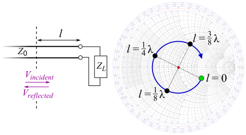
Using transmission-line theory, if a transmission line is terminated in an impedance (${\displaystyle Z_{\text{T}}\,}$) which differs from its characteristic impedance (${\displaystyle Z_{0}\,}$), a standing wave will be formed on the line comprising the resultant of both the incident or forward (${\displaystyle V_{\text{F}}\,}$) and the reflected or reversed (${\displaystyle V_{\text{R}}\,}$) waves. Using complex exponential notation:

${\displaystyle V_{\text{F}}=A\exp(j\omega t)\exp(+\gamma \ell )~\,}$ and

${\displaystyle V_{\text{R}}=B\exp(j\omega t)\exp(-\gamma \ell )\,}$

where

${\displaystyle \exp(j\omega t)\,}$ is the temporal part of the wave

${\displaystyle \exp(\pm \gamma \ell )\,}$ is the spatial part of the wave and

${\displaystyle \omega =2\pi f\,}$ where

${\displaystyle \omega \,}$ is the angular frequency in radians per second (rad/s)

${\displaystyle f\,}$ is the frequency in hertz (Hz)

${\displaystyle t\,}$ is the time in seconds (s)

${\displaystyle A\,}$ and ${\displaystyle B\,}$ are constants

${\displaystyle \ell \,}$ is the distance measured along the transmission line from the load toward the generator in metres (m)

Also

${\displaystyle \gamma =\alpha +j\beta \,}$ is the propagation constant which has units 1/m

where

${\displaystyle \alpha \,}$ is the attenuation constant in nepers per metre (Np/m)

${\displaystyle \beta \,}$ is the phase constant in radians per metre (rad/m)

The Smith chart is used with one frequency (${\displaystyle \omega }$) at a time, and only for one moment (${\displaystyle t}$) at a time, so the temporal part of the phase (${\displaystyle \exp(j\omega t)\,}$) is fixed. All terms are actually multiplied by this to obtain the instantaneous phase, but it is conventional and understood to omit it. Therefore,

${\displaystyle V_{\text{F}}=A\exp(+\gamma \ell )\,}$ and

${\displaystyle V_{\text{R}}=B\exp(-\gamma \ell )\,}$

where ${\displaystyle A\,}$ and ${\displaystyle B\,}$ are respectively the forward and reverse voltage amplitudes at the load.

The variation of complex reflection coefficient with position along the line[]

Looking towards a load through a length ${\displaystyle \ell \,}$ of lossless transmission line, the impedance changes as ${\displaystyle \ell \,}$ increases, following the blue circle. (This impedance is characterized by its reflection coefficient ${\displaystyle V_{\text{reflected}}/V_{\text{incident}}}$.) The blue circle, centered within the impedance Smith chart, is sometimes called an SWR circle (short for constant standing wave ratio).

The complex voltage reflection coefficient ${\displaystyle \Gamma \,}$ is defined as the ratio of the reflected wave to the incident (or forward) wave. Therefore,

${\displaystyle \Gamma ={\frac {V_{\text{R}}}{V_{\text{F}}}}={\frac {B\exp(-\gamma \ell )}{A\exp(+\gamma \ell )}}=C\exp(-2\gamma \ell )\,}$

where C is also a constant.

For a uniform transmission line (in which ${\displaystyle \gamma \,}$ is constant), the complex reflection coefficient of a standing wave varies according to the position on the line. If the line is lossy (${\displaystyle \alpha \,}$ is non-zero) this is represented on the Smith chart by a spiral path. In most Smith chart problems however, losses can be assumed negligible (${\displaystyle \alpha =0\,}$) and the task of solving them is greatly simplified. For the loss free case therefore, the expression for complex reflection coefficient becomes

${\displaystyle \Gamma =\Gamma _{\text{L}}\exp(-2j\beta \ell )\,}$

where ${\displaystyle \Gamma _{\text{L}}\,}$ is the reflection coefficient at the load, and ${\displaystyle \ell \,}$ is the line length from the load to the location where the reflection coefficient is measured. The phase constant ${\displaystyle \beta \,}$ may also be written as

${\displaystyle \beta ={\frac {2\pi }{\lambda }}\,}$

where ${\displaystyle \lambda \,}$ is the wavelength within the transmission line at the test frequency.

Therefore,

${\displaystyle \Gamma =\Gamma _{\text{L}}\exp \left({\frac {-4j\pi }{\lambda }}\ell \right)\,}$

This equation shows that, for a standing wave, the complex reflection coefficient and impedance repeats every half wavelength along the transmission line. The complex reflection coefficient is generally simply referred to as reflection coefficient. The outer circumferential scale of the Smith chart represents the distance from the generator to the load scaled in wavelengths and is therefore scaled from zero to 0.50 .

The variation of normalised impedance with position along the line[]

If ${\displaystyle V\,}$ and ${\displaystyle I\,}$ are the voltage across and the current entering the termination at the end of the transmission line respectively, then

${\displaystyle V_{\text{F}}+V_{\text{R}}=V\,}$ and

${\displaystyle V_{\text{F}}-V_{\text{R}}=Z_{0}I\,}$.

By dividing these equations and substituting for both the voltage reflection coefficient

${\displaystyle \Gamma ={\frac {V_{\text{R}}}{V_{\text{F}}}}\,}$

and the normalised impedance of the termination represented by the lower case z, subscript T

${\displaystyle z_{\text{T}}={\frac {V}{Z_{0}I}}\,}$

gives the result:

${\displaystyle z_{\text{T}}={\frac {1+\Gamma }{1-\Gamma }}\,}$.

Alternatively, in terms of the reflection coefficient

${\displaystyle \Gamma ={\frac {z_{\text{T}}-1}{z_{\text{T}}+1}}\,}$

These are the equations which are used to construct the Z Smith chart. Mathematically speaking ${\displaystyle \Gamma \,}$ and ${\displaystyle z_{\text{T}}\,}$ are related via a Möbius transformation.

Both ${\displaystyle \Gamma \,}$ and ${\displaystyle z_{\text{T}}\,}$ are expressed in complex numbers without any units. They both change with frequency so for any particular measurement, the frequency at which it was performed must be stated together with the characteristic impedance.

${\displaystyle \Gamma \,}$ may be expressed in magnitude and angle on a polar diagram. Any actual reflection coefficient must have a magnitude of less than or equal to unity so, at the test frequency, this may be expressed by a point inside a circle of unity radius. The Smith chart is actually constructed on such a polar diagram. The Smith chart scaling is designed in such a way that reflection coefficient can be converted to normalised impedance or vice versa. Using the Smith chart, the normalised impedance may be obtained with appreciable accuracy by plotting the point representing the reflection coefficient treating the Smith chart as a polar diagram and then reading its value directly using the characteristic Smith chart scaling. This technique is a graphical alternative to substituting the values in the equations.

By substituting the expression for how reflection coefficient changes along an unmatched loss-free transmission line

${\displaystyle \Gamma ={\frac {B\exp(-\gamma \ell )}{A\exp(\gamma \ell )}}={\frac {B\exp(-j\beta \ell )}{A\exp(j\beta \ell )}}\,}$

for the loss free case, into the equation for normalised impedance in terms of reflection coefficient

${\displaystyle z_{\text{T}}={\frac {1+\Gamma }{1-\Gamma }}\,}$.

and using Euler's formula

${\displaystyle \exp(j\theta )=\cos \theta +j\sin \theta \,}$

yields the impedance-version transmission-line equation for the loss free case:^[11]

${\displaystyle Z_{\text{in}}=Z_{0}{\frac {Z_{\text{L}}+jZ_{0}\tan(\beta \ell )}{Z_{0}+jZ_{\text{L}}\tan(\beta \ell )}}\,}$

where ${\displaystyle Z_{\text{in}}\,}$ is the impedance 'seen' at the input of a loss free transmission line of length ${\displaystyle \ell }$, terminated with an impedance ${\displaystyle Z_{\text{L}}\,}$

Versions of the transmission-line equation may be similarly derived for the admittance loss free case and for the impedance and admittance lossy cases.

The Smith chart graphical equivalent of using the transmission-line equation is to normalise ${\displaystyle Z_{\text{L}}\,}$, to plot the resulting point on a Z Smith chart and to draw a circle through that point centred at the Smith chart centre. The path along the arc of the circle represents how the impedance changes whilst moving along the transmission line. In this case the circumferential (wavelength) scaling must be used, remembering that this is the wavelength within the transmission line and may differ from the free space wavelength.

Regions of the Z Smith chart[]

If a polar diagram is mapped on to a cartesian coordinate system it is conventional to measure angles relative to the positive x-axis using a counterclockwise direction for positive angles. The magnitude of a complex number is the length of a straight line drawn from the origin to the point representing it. The Smith chart uses the same convention, noting that, in the normalised impedance plane, the positive x-axis extends from the center of the Smith chart at ${\displaystyle z_{\text{T}}=1\pm j0\,}$ to the point ${\displaystyle z_{\text{T}}=\infty \pm j\infty \,}$. The region above the x-axis represents inductive impedances (positive imaginary parts) and the region below the x-axis represents capacitive impedances (negative imaginary parts).

If the termination is perfectly matched, the reflection coefficient will be zero, represented effectively by a circle of zero radius or in fact a point at the centre of the Smith chart. If the termination was a perfect open circuit or short circuit the magnitude of the reflection coefficient would be unity, all power would be reflected and the point would lie at some point on the unity circumference circle.

Circles of constant normalised resistance and constant normalised reactance[]

The normalised impedance Smith chart is composed of two families of circles: circles of constant normalised resistance and circles of constant normalised reactance. In the complex reflection coefficient plane the Smith chart occupies a circle of unity radius centred at the origin. In cartesian coordinates therefore the circle would pass through the points (+1,0) and (−1,0) on the x-axis and the points (0,+1) and (0,−1) on the y-axis.

Since both ${\displaystyle \Gamma }$ and ${\displaystyle z\,}$ are complex numbers, in general they may be written as:

${\displaystyle z=a+jb\,}$

${\displaystyle \Gamma =c+jd\,}$

with a, b, c and d real numbers.

Substituting these into the equation relating normalised impedance and complex reflection coefficient:

${\displaystyle \Gamma ={\frac {z-1}{z+1}}\,}$

gives the following result:

${\displaystyle \Gamma =c+jd=\left[{\frac {a^{2}+b^{2}-1}{(a+1)^{2}+b^{2}}}\right]+j\left[{\frac {2b}{(a+1)^{2}+b^{2}}}\right]\,}$.

This is the equation which describes how the complex reflection coefficient changes with the normalised impedance and may be used to construct both families of circles.^[12]

The Y Smith chart[]

The Y Smith chart is constructed in a similar way to the Z Smith chart case but by expressing values of voltage reflection coefficient in terms of normalised admittance instead of normalised impedance. The normalised admittance y_T is the reciprocal of the normalised impedance z_T, so

${\displaystyle y_{\text{T}}={\frac {1}{z_{\text{T}}}}\,}$

Therefore:

${\displaystyle y_{\text{T}}={\frac {1-\Gamma }{1+\Gamma }}\,}$

and

${\displaystyle \Gamma ={\frac {1-y_{\text{T}}}{1+y_{\text{T}}}}\,}$

The Y Smith chart appears like the normalised impedance type but with the graphic scaling rotated through 180°, the numeric scaling remaining unchanged.

The region above the x-axis represents capacitive admittances and the region below the x-axis represents inductive admittances. Capacitive admittances have positive imaginary parts and inductive admittances have negative imaginary parts.

Again, if the termination is perfectly matched the reflection coefficient will be zero, represented by a 'circle' of zero radius or in fact a point at the centre of the Smith chart. If the termination was a perfect open or short circuit the magnitude of the voltage reflection coefficient would be unity, all power would be reflected and the point would lie at some point on the unity circumference circle of the Smith chart.

Practical examples[]

Example points plotted on the normalised impedance Smith chart

A point with a reflection coefficient magnitude 0.63 and angle 60° represented in polar form as ${\displaystyle 0.63\angle 60^{\circ }\,}$, is shown as point P₁ on the Smith chart. To plot this, one may use the circumferential (reflection coefficient) angle scale to find the ${\displaystyle \angle 60^{\circ }\,}$ graduation and a ruler to draw a line passing through this and the centre of the Smith chart. The length of the line would then be scaled to P₁ assuming the Smith chart radius to be unity. For example, if the actual radius measured from the paper was 100 mm, the length OP₁ would be 63 mm.

The following table gives some similar examples of points which are plotted on the Z Smith chart. For each, the reflection coefficient is given in polar form together with the corresponding normalised impedance in rectangular form. The conversion may be read directly from the Smith chart or by substitution into the equation.

Some examples of points plotted on the normalised impedance Smith chart

Point identity	Reflection coefficient (polar form)	Normalised impedance (rectangular form)
P1 (Inductive)	${\displaystyle 0.63\angle 60^{\circ }\,}$	${\displaystyle 0.80+j1.40\,}$
P2 (Inductive)	${\displaystyle 0.73\angle 125^{\circ }\,}$	${\displaystyle 0.20+j0.50\,}$
P3 (Capacitive)	${\displaystyle 0.44\angle -116^{\circ }\,}$	${\displaystyle 0.50-j0.50\,}$

Working with both the Z Smith chart and the Y Smith charts[]

In RF circuit and matching problems sometimes it is more convenient to work with admittances (representing conductances and susceptances) and sometimes it is more convenient to work with impedances (representing resistances and reactances). Solving a typical matching problem will often require several changes between both types of Smith chart, using normalised impedance for series elements and normalised admittances for parallel elements. For these a dual (normalised) impedance and admittance Smith chart may be used. Alternatively, one type may be used and the scaling converted to the other when required. In order to change from normalised impedance to normalised admittance or vice versa, the point representing the value of reflection coefficient under consideration is moved through exactly 180 degrees at the same radius. For example, the point P1 in the example representing a reflection coefficient of ${\displaystyle 0.63\angle 60^{\circ }\,}$ has a normalised impedance of ${\displaystyle z_{P}=0.80+j1.40\,}$. To graphically change this to the equivalent normalised admittance point, say Q1, a line is drawn with a ruler from P1 through the Smith chart centre to Q1, an equal radius in the opposite direction. This is equivalent to moving the point through a circular path of exactly 180 degrees. Reading the value from the Smith chart for Q1, remembering that the scaling is now in normalised admittance, gives ${\displaystyle y_{P}=0.30-j0.54\,}$. Performing the calculation

${\displaystyle y_{\text{T}}={\frac {1}{z_{\text{T}}}}\,}$

manually will confirm this.

Once a transformation from impedance to admittance has been performed, the scaling changes to normalised admittance until a later transformation back to normalised impedance is performed.

The table below shows examples of normalised impedances and their equivalent normalised admittances obtained by rotation of the point through 180°. Again, these may be obtained either by calculation or using a Smith chart as shown, converting between the normalised impedance and normalised admittances planes.

Values of reflection coefficient as normalised impedances and the equivalent normalised admittances

Normalised Impedance Plane	Normalised Admittance Plane
P1 (${\displaystyle z=0.80+j1.40\,}$)	Q1 (${\displaystyle y=0.30-j0.54\,}$)
P10 (${\displaystyle z=0.10+j0.22\,}$)	Q10 (${\displaystyle y=1.80-j3.90\,}$)

Values of complex reflection coefficient plotted on the normalised impedance Smith chart and their equivalents on the normalised admittance Smith chart

Choice of Smith chart type and component type[]

The choice of whether to use the Z Smith chart or the Y Smith chart for any particular calculation depends on which is more convenient. Impedances in series and admittances in parallel add while impedances in parallel and admittances in series are related by a reciprocal equation. If ${\displaystyle Z_{\text{TS}}}$ is the equivalent impedance of series impedances and ${\displaystyle Z_{\text{TP}}}$ is the equivalent impedance of parallel impedances, then

${\displaystyle Z_{\text{TS}}=Z_{1}+Z_{2}+Z_{3}+...\,}$

${\displaystyle {\frac {1}{Z_{\text{TP}}}}={\frac {1}{Z_{1}}}+{\frac {1}{Z_{2}}}+{\frac {1}{Z_{3}}}+...\,}$

For admittances the reverse is true, that is

${\displaystyle Y_{\text{TP}}=Y_{1}+Y_{2}+Y_{3}+...\,}$

${\displaystyle {\frac {1}{Y_{\text{TS}}}}={\frac {1}{Y_{1}}}+{\frac {1}{Y_{2}}}+{\frac {1}{Y_{3}}}+...\,}$

Dealing with the reciprocals, especially in complex numbers, is more time consuming and error-prone than using linear addition. In general therefore, most RF engineers work in the plane where the circuit topography supports linear addition. The following table gives the complex expressions for impedance (real and normalised) and admittance (real and normalised) for each of the three basic passive circuit elements: resistance, inductance and capacitance. Using just the characteristic impedance (or characteristic admittance) and test frequency an equivalent circuit can be found and vice versa.

Expressions for Impedance and Admittance
Normalised by Impedance Z₀ or Admittance Y₀

Element Type	Impedance (Z or z) or Reactance (X or x)		Admittance (Y or y) or Susceptance (B or b)
	Real (${\displaystyle \Omega \,}$)	Normalised (No Unit)	Real (S)	Normalised (No Unit)
Resistance (R)	${\displaystyle Z=R\,}$	${\displaystyle z={\frac {R}{Z_{0}}}=RY_{0}\,}$	${\displaystyle Y=G={\frac {1}{R}}\,}$	${\displaystyle y=g={\frac {1}{RY_{0}}}={\frac {Z_{0}}{R}}\,}$
Inductance (L)	${\displaystyle Z=jX_{\text{L}}=j\omega L\,}$	${\displaystyle z=jx_{\text{L}}=j{\frac {\omega L}{Z_{0}}}=j\omega LY_{0}\,}$	${\displaystyle Y=-jB_{\text{L}}={\frac {-j}{\omega L}}}$	${\displaystyle y=-jb_{\text{L}}={\frac {-j}{\omega LY_{0}}}={\frac {-jZ_{0}}{\omega L}}\,}$
Capacitance (C)	${\displaystyle Z=-jX_{\text{C}}={\frac {-j}{\omega C}}\,}$	${\displaystyle z=-jx_{\text{C}}={\frac {-j}{\omega CZ_{0}}}={\frac {-jY_{0}}{\omega C}}\,}$	${\displaystyle Y=jB_{\text{C}}=j\omega C\,}$	${\displaystyle y=jb_{\text{C}}=j{\frac {\omega C}{Y_{0}}}=j\omega CZ_{0}\,}$

Using the Smith chart to solve conjugate matching problems with distributed components[]

Distributed matching becomes feasible and is sometimes required when the physical size of the matching components is more than about 5% of a wavelength at the operating frequency. Here the electrical behaviour of many lumped components becomes rather unpredictable. This occurs in microwave circuits and when high power requires large components in shortwave, FM and TV Broadcasting,

For distributed components the effects on reflection coefficient and impedance of moving along the transmission line must be allowed for using the outer circumferential scale of the Smith chart which is calibrated in wavelengths.

The following example shows how a transmission line, terminated with an arbitrary load, may be matched at one frequency either with a series or parallel reactive component in each case connected at precise positions.

Smith chart construction for some distributed transmission-line matching

Supposing a loss-free air-spaced transmission line of characteristic impedance ${\displaystyle Z_{0}=50\ \Omega }$, operating at a frequency of 800 MHz, is terminated with a circuit comprising a 17.5 ${\displaystyle \Omega }$ resistor in series with a 6.5 nanohenry (6.5 nH) inductor. How may the line be matched?

From the table above, the reactance of the inductor forming part of the termination at 800 MHz is

${\displaystyle Z_{L}=j\omega L=j2\pi fL=j32.7\ \Omega \,}$

so the impedance of the combination (${\displaystyle Z_{T}}$) is given by

${\displaystyle Z_{T}=17.5+j32.7\ \Omega \,}$

and the normalised impedance (${\displaystyle z_{T}}$) is

${\displaystyle z_{T}={\frac {Z_{T}}{Z_{0}}}=0.35+j0.65\,}$

This is plotted on the Z Smith chart at point P₂₀. The line OP₂₀ is extended through to the wavelength scale where it intersects at the point ${\displaystyle L_{1}=0.098\lambda \,}$. As the transmission line is loss free, a circle centred at the centre of the Smith chart is drawn through the point P₂₀ to represent the path of the constant magnitude reflection coefficient due to the termination. At point P₂₁ the circle intersects with the unity circle of constant normalised resistance at

${\displaystyle z_{P21}=1.00+j1.52\,}$.

The extension of the line OP₂₁ intersects the wavelength scale at ${\displaystyle L_{2}=0.177\lambda \,}$, therefore the distance from the termination to this point on the line is given by

${\displaystyle L_{2}-L_{1}=0.177\lambda -0.098\lambda =0.079\lambda \,}$

Since the transmission line is air-spaced, the wavelength at 800 MHz in the line is the same as that in free space and is given by

${\displaystyle \lambda ={\frac {c}{f}}\,}$

where ${\displaystyle c\,}$ is the velocity of electromagnetic radiation in free space and ${\displaystyle f\,}$ is the frequency in hertz. The result gives ${\displaystyle \lambda =375\ \mathrm {mm} \,}$, making the position of the matching component 29.6 mm from the load.

The conjugate match for the impedance at P₂₁ (${\displaystyle z_{match}\,}$) is

${\displaystyle z_{match}=-j(1.52),\!}$

As the Smith chart is still in the normalised impedance plane, from the table above a series capacitor ${\displaystyle C_{m}\,}$ is required where

${\displaystyle z_{match}=-j1.52={\frac {-j}{\omega C_{m}Z_{0}}}={\frac {-j}{2\pi fC_{m}Z_{0}}}\,}$

Rearranging, we obtain

${\displaystyle C_{m}={\frac {1}{(1.52)\omega Z_{0}}}={\frac {1}{(1.52)(2\pi f)Z_{0}}}}$.

Substitution of known values gives

${\displaystyle C_{m}=2.6\ \mathrm {pF} \,}$

To match the termination at 800 MHz, a series capacitor of 2.6 pF must be placed in series with the transmission line at a distance of 29.6 mm from the termination.

An alternative shunt match could be calculated after performing a Smith chart transformation from normalised impedance to normalised admittance. Point Q₂₀ is the equivalent of P₂₀ but expressed as a normalised admittance. Reading from the Smith chart scaling, remembering that this is now a normalised admittance gives

${\displaystyle y_{Q20}=0.65-j1.20\,}$

(In fact this value is not actually used). However, the extension of the line OQ₂₀ through to the wavelength scale gives ${\displaystyle L_{3}=0.152\lambda \,}$. The earliest point at which a shunt conjugate match could be introduced, moving towards the generator, would be at Q₂₁, the same position as the previous P₂₁, but this time representing a normalised admittance given by

${\displaystyle y_{Q21}=1.00+j1.52\,}$.

The distance along the transmission line is in this case

${\displaystyle L_{2}+L_{3}=0.177\lambda +0.152\lambda =0.329\lambda \,}$

which converts to 123 mm.

The conjugate matching component is required to have a normalised admittance (${\displaystyle y_{match}}$) of

${\displaystyle y_{match}=-j1.52\,}$.

From the table it can be seen that a negative admittance would require an inductor, connected in parallel with the transmission line. If its value is ${\displaystyle L_{m}\,}$, then

${\displaystyle -j1.52={\frac {-j}{\omega L_{m}Y_{0}}}={\frac {-jZ_{0}}{2\pi fL_{m}}}\,}$

This gives the result

${\displaystyle L_{m}=6.5\ \mathrm {nH} \,}$

A suitable inductive shunt matching would therefore be a 6.5 nH inductor in parallel with the line positioned at 123 mm from the load.

Using the Smith chart to analyze lumped-element circuits[]

The analysis of lumped-element components assumes that the wavelength at the frequency of operation is much greater than the dimensions of the components themselves. The Smith chart may be used to analyze such circuits in which case the movements around the chart are generated by the (normalized) impedances and admittances of the components at the frequency of operation. In this case the wavelength scaling on the Smith chart circumference is not used. The following circuit will be analyzed using a Smith chart at an operating frequency of 100 MHz. At this frequency the free space wavelength is 3 m. The component dimensions themselves will be in the order of millimetres so the assumption of lumped components will be valid. Despite there being no transmission line as such, a system impedance must still be defined to enable normalization and de-normalization calculations and ${\displaystyle Z_{0}=50\ \Omega \,}$ is a good choice here as ${\displaystyle R_{1}=50\ \Omega \,}$. If there were very different values of resistance present a value closer to these might be a better choice.

A lumped-element circuit which may be analysed using a Smith chart

Smith chart with graphical construction for analysis of a lumped circuit

The analysis starts with a Z Smith chart looking into R₁ only with no other components present. As ${\displaystyle R_{1}=50\ \Omega \,}$ is the same as the system impedance, this is represented by a point at the centre of the Smith chart. The first transformation is OP₁ along the line of constant normalized resistance in this case the addition of a normalized reactance of -j0.80, corresponding to a series capacitor of 40 pF. Points with suffix P are in the Z plane and points with suffix Q are in the Y plane. Therefore, transformations P₁ to Q₁ and P₃ to Q₃ are from the Z Smith chart to the Y Smith chart and transformation Q₂ to P₂ is from the Y Smith chart to the Z Smith chart. The following table shows the steps taken to work through the remaining components and transformations, returning eventually back to the centre of the Smith chart and a perfect 50 ohm match.

Smith chart steps for analysing a lumped-element circuit

Transformation	Plane	x or y Normalized Value	Capacitance/Inductance	Formula to Solve	Result
${\displaystyle O\rightarrow P_{1}\,}$	${\displaystyle Z\,}$	${\displaystyle -j0.80\,}$	Capacitance (Series)	${\displaystyle -j0.80={\frac {-j}{\omega C_{1}Z_{0}}}\,}$	${\displaystyle C_{1}=40\ \mathrm {pF} \,}$
${\displaystyle Q_{1}\rightarrow Q_{2}\,}$	${\displaystyle Y\,}$	${\displaystyle -j1.49\,}$	Inductance (Shunt)	${\displaystyle -j1.49={\frac {-j}{\omega L_{1}Y_{0}}}\,}$	${\displaystyle L_{1}=53\ \mathrm {nH} \,}$
${\displaystyle P_{2}\rightarrow P_{3}\,}$	Z	${\displaystyle -j0.23\,}$	Capacitance (Series)	${\displaystyle -j0.23={\frac {-j}{\omega C_{2}Z_{0}}}\,}$	${\displaystyle C_{2}=138\ \mathrm {pF} \,}$
${\displaystyle Q_{3}\rightarrow O\,}$	Y	${\displaystyle +j1.14\,}$	Capacitance (Shunt)	${\displaystyle +j1.14={\frac {j\omega C_{3}}{Y_{0}}}\,}$	${\displaystyle C_{3}=36\ \mathrm {pF} \,}$

3D Smith chart[]

3D Smith chart representation

A generalized 3D Smith chart based on the extended complex plane (Riemann sphere) and inversive geometry was proposed in 2011. The chart unifies the passive and active circuit design on little and big circles on the surface of a unit sphere using the stereographic conformal map of the reflection coefficient's generalized plane. Considering the point at infinity, the space of the new chart includes all possible loads. The north pole is the perfect matching point, while the south pole is the perfect mismatch point.^[13] The 3D Smith chart has been further extended outside of the spherical surface, for plotting various scalar parameters such as group delay, quality factors or frequency orientation. The frequency orientation visualization (clockwise/counter-clockwise) enables one to differentiate between a negative capacitance and positive inductor whose reflection coefficients are the same when plotted on a 2D Smith chart, but whose orientations diverge as frequency increases.^[14]

References[]

Further reading[]

• For an early representation of this graphical depiction before they were called 'Smith Charts', see Campbell, G. A. (1911). "Cisoidal oscillations". Proceedings of the American Institute of Electrical Engineers. 30 (1–6): 789–824. doi:10.1109/PAIEE.1911.6659711., In particular, Fig. 13 on p. 810.

External links[]

Wikimedia Commons has media related to Smith charts.

• "Mathematical construction and properties of the Smith Chart". allaboutcircuits.com. technical articles.
• "Smith Chart and Impedance Matching Tutorial with Examples". antenna-theory.com.
• "The Mizuhashi-Smith chart". www.linkclub.or.jp/~morikuni. Archived from the original on 2013-03-03.
• "Excel Smith chart". excelhero.com. August 2010. Non-commercial, interactive Smith Chart that looks best in Excel 2007+.
• "SimSmith". ae6ty.com. Non-commercial, available for Windows, Mac, and Linux. Many Smith chart tutorial videos. No circuit size restrictions. Not limited to ladder circuits.
• "Smith v3". fritz.dellsperger.net. Archived from the original on 2015-03-04. Commercial and free Smith chart for Windows
• "QuickSmith". github.com/niyeradori. Free web based Smith Chart Educational tool available on GitHub.
• "3D Smith chart tool". 3dsmithchart.com. 2D and 3D Smith chart generalized tool for active and passive circuits (free for academia/education).