Covariance matrix

Part of a series on Statistics
Correlation and covariance
hide For random vectors Autocorrelation matrix Cross-correlation matrix Auto-covariance matrix Cross-covariance matrix
hide For stochastic processes Autocorrelation function Cross-correlation function Autocovariance function Cross-covariance function
hide For deterministic signals Autocorrelation function Cross-correlation function Autocovariance function
v t

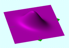
A bivariate Gaussian probability density function centered at (0, 0), with covariance matrix given by ${\displaystyle {\begin{bmatrix}1&0.5\\0.5&1\end{bmatrix}}}$

Sample points from a bivariate Gaussian distribution with a standard deviation of 3 in roughly the lower left-upper right direction and of 1 in the orthogonal direction. Because the x and y components co-vary, the variances of ${\displaystyle x}$ and ${\displaystyle y}$ do not fully describe the distribution. A ${\displaystyle 2\times 2}$ covariance matrix is needed; the directions of the arrows correspond to the eigenvectors of this covariance matrix and their lengths to the square roots of the eigenvalues.

In probability theory and statistics, a covariance matrix (also known as auto-covariance matrix, dispersion matrix, variance matrix, or variance–covariance matrix) is a square matrix giving the covariance between each pair of elements of a given random vector. Any covariance matrix is symmetric and positive semi-definite and its main diagonal contains variances (i.e., the covariance of each element with itself).

Intuitively, the covariance matrix generalizes the notion of variance to multiple dimensions. As an example, the variation in a collection of random points in two-dimensional space cannot be characterized fully by a single number, nor would the variances in the ${\displaystyle x}$ and ${\displaystyle y}$ directions contain all of the necessary information; a ${\displaystyle 2\times 2}$ matrix would be necessary to fully characterize the two-dimensional variation.

The covariance matrix of a random vector ${\displaystyle \mathbf {X} }$ is typically denoted by ${\displaystyle \operatorname {K} _{\mathbf {X} \mathbf {X} }}$ or ${\displaystyle \Sigma }$.

Definition[]

Throughout this article, boldfaced unsubscripted ${\displaystyle \mathbf {X} }$ and ${\displaystyle \mathbf {Y} }$ are used to refer to random vectors, and unboldfaced subscripted ${\displaystyle X_{i}}$ and ${\displaystyle Y_{i}}$ are used to refer to scalar random variables.

If the entries in the column vector

${\displaystyle \mathbf {X} =(X_{1},X_{2},...,X_{n})^{\mathrm {T} }}$

are random variables, each with finite variance and expected value, then the covariance matrix ${\displaystyle \operatorname {K} _{\mathbf {X} \mathbf {X} }}$ is the matrix whose ${\displaystyle (i,j)}$ entry is the covariance^{[1]: p. 177}

${\displaystyle \operatorname {K} _{X_{i}X_{j}}=\operatorname {cov} [X_{i},X_{j}]=\operatorname {E} [(X_{i}-\operatorname {E} [X_{i}])(X_{j}-\operatorname {E} [X_{j}])]}$

where the operator ${\displaystyle \operatorname {E} }$ denotes the expected value (mean) of its argument.

In other words,

${\displaystyle \operatorname {K} _{\mathbf {X} \mathbf {X} }={\begin{bmatrix}\mathrm {E} [(X_{1}-\operatorname {E} [X_{1}])(X_{1}-\operatorname {E} [X_{1}])]&\mathrm {E} [(X_{1}-\operatorname {E} [X_{1}])(X_{2}-\operatorname {E} [X_{2}])]&\cdots &\mathrm {E} [(X_{1}-\operatorname {E} [X_{1}])(X_{n}-\operatorname {E} [X_{n}])]\\\\\mathrm {E} [(X_{2}-\operatorname {E} [X_{2}])(X_{1}-\operatorname {E} [X_{1}])]&\mathrm {E} [(X_{2}-\operatorname {E} [X_{2}])(X_{2}-\operatorname {E} [X_{2}])]&\cdots &\mathrm {E} [(X_{2}-\operatorname {E} [X_{2}])(X_{n}-\operatorname {E} [X_{n}])]\\\\\vdots &\vdots &\ddots &\vdots \\\\\mathrm {E} [(X_{n}-\operatorname {E} [X_{n}])(X_{1}-\operatorname {E} [X_{1}])]&\mathrm {E} [(X_{n}-\operatorname {E} [X_{n}])(X_{2}-\operatorname {E} [X_{2}])]&\cdots &\mathrm {E} [(X_{n}-\operatorname {E} [X_{n}])(X_{n}-\operatorname {E} [X_{n}])]\end{bmatrix}}}$

The definition above is equivalent to the matrix equality

${\displaystyle \operatorname {K} _{\mathbf {X} \mathbf {X} }=\operatorname {cov} [\mathbf {X} ,\mathbf {X} ]=\operatorname {E} [(\mathbf {X} -\mathbf {\mu _{X}} )(\mathbf {X} -\mathbf {\mu _{X}} )^{\rm {T}}]=\operatorname {E} [\mathbf {X} \mathbf {X} ^{T}]-\mathbf {\mu _{X}} \mathbf {\mu _{X}} ^{T}}$

(Eq.1)

where ${\displaystyle \mathbf {\mu _{X}} =\operatorname {E} [\mathbf {X} ]}$.

Generalization of the variance[]

This form (Eq.1) can be seen as a generalization of the scalar-valued variance to higher dimensions. Remember that for a scalar-valued random variable ${\displaystyle X}$

${\displaystyle \sigma _{X}^{2}=\operatorname {var} (X)=\operatorname {E} [(X-\operatorname {E} [X])^{2}]=\operatorname {E} [(X-\operatorname {E} [X])\cdot (X-\operatorname {E} [X])].}$

Indeed, the entries on the diagonal of the auto-covariance matrix ${\displaystyle \operatorname {K} _{\mathbf {X} \mathbf {X} }}$ are the variances of each element of the vector ${\displaystyle \mathbf {X} }$.

Conflicting nomenclatures and notations[]

Nomenclatures differ. Some statisticians, following the probabilist William Feller in his two-volume book An Introduction to Probability Theory and Its Applications,^[2] call the matrix ${\displaystyle \operatorname {K} _{\mathbf {X} \mathbf {X} }}$ the variance of the random vector ${\displaystyle \mathbf {X} }$, because it is the natural generalization to higher dimensions of the 1-dimensional variance. Others call it the covariance matrix, because it is the matrix of covariances between the scalar components of the vector ${\displaystyle \mathbf {X} }$.

${\displaystyle \operatorname {var} (\mathbf {X} )=\operatorname {cov} (\mathbf {X} )=\operatorname {E} \left[(\mathbf {X} -\operatorname {E} [\mathbf {X} ])(\mathbf {X} -\operatorname {E} [\mathbf {X} ])^{\rm {T}}\right].}$

Both forms are quite standard, and there is no ambiguity between them. The matrix ${\displaystyle \operatorname {K} _{\mathbf {X} \mathbf {X} }}$ is also often called the variance-covariance matrix, since the diagonal terms are in fact variances.

By comparison, the notation for the cross-covariance matrix between two vectors is

${\displaystyle \operatorname {cov} (\mathbf {X} ,\mathbf {Y} )=\operatorname {K} _{\mathbf {X} \mathbf {Y} }=\operatorname {E} \left[(\mathbf {X} -\operatorname {E} [\mathbf {X} ])(\mathbf {Y} -\operatorname {E} [\mathbf {Y} ])^{\rm {T}}\right].}$

Properties[]

Relation to the autocorrelation matrix[]

The auto-covariance matrix ${\displaystyle \operatorname {K} _{\mathbf {X} \mathbf {X} }}$ is related to the autocorrelation matrix ${\displaystyle \operatorname {R} _{\mathbf {X} \mathbf {X} }}$ by

${\displaystyle \operatorname {K} _{\mathbf {X} \mathbf {X} }=\operatorname {E} [(\mathbf {X} -\operatorname {E} [\mathbf {X} ])(\mathbf {X} -\operatorname {E} [\mathbf {X} ])^{\rm {T}}]=\operatorname {R} _{\mathbf {X} \mathbf {X} }-\operatorname {E} [\mathbf {X} ]\operatorname {E} [\mathbf {X} ]^{\rm {T}}}$

where the autocorrelation matrix is defined as ${\displaystyle \operatorname {R} _{\mathbf {X} \mathbf {X} }=\operatorname {E} [\mathbf {X} \mathbf {X} ^{\rm {T}}]}$.

Relation to the correlation matrix[]

An entity closely related to the covariance matrix is the matrix of Pearson product-moment correlation coefficients between each of the random variables in the random vector ${\displaystyle \mathbf {X} }$, which can be written as

${\displaystyle \operatorname {corr} (\mathbf {X} )={\big (}\operatorname {diag} (\operatorname {K} _{\mathbf {X} \mathbf {X} }){\big )}^{-{\frac {1}{2}}}\,\operatorname {K} _{\mathbf {X} \mathbf {X} }\,{\big (}\operatorname {diag} (\operatorname {K} _{\mathbf {X} \mathbf {X} }){\big )}^{-{\frac {1}{2}}},}$

where ${\displaystyle \operatorname {diag} (\operatorname {K} _{\mathbf {X} \mathbf {X} })}$ is the matrix of the diagonal elements of ${\displaystyle \operatorname {K} _{\mathbf {X} \mathbf {X} }}$ (i.e., a diagonal matrix of the variances of ${\displaystyle X_{i}}$ for ${\displaystyle i=1,\dots ,n}$).

Equivalently, the correlation matrix can be seen as the covariance matrix of the standardized random variables ${\displaystyle X_{i}/\sigma (X_{i})}$ for ${\displaystyle i=1,\dots ,n}$.

${\displaystyle \operatorname {corr} (\mathbf {X} )={\begin{bmatrix}1&{\frac {\operatorname {E} [(X_{1}-\mu _{1})(X_{2}-\mu _{2})]}{\sigma (X_{1})\sigma (X_{2})}}&\cdots &{\frac {\operatorname {E} [(X_{1}-\mu _{1})(X_{n}-\mu _{n})]}{\sigma (X_{1})\sigma (X_{n})}}\\\\{\frac {\operatorname {E} [(X_{2}-\mu _{2})(X_{1}-\mu _{1})]}{\sigma (X_{2})\sigma (X_{1})}}&1&\cdots &{\frac {\operatorname {E} [(X_{2}-\mu _{2})(X_{n}-\mu _{n})]}{\sigma (X_{2})\sigma (X_{n})}}\\\\\vdots &\vdots &\ddots &\vdots \\\\{\frac {\operatorname {E} [(X_{n}-\mu _{n})(X_{1}-\mu _{1})]}{\sigma (X_{n})\sigma (X_{1})}}&{\frac {\operatorname {E} [(X_{n}-\mu _{n})(X_{2}-\mu _{2})]}{\sigma (X_{n})\sigma (X_{2})}}&\cdots &1\end{bmatrix}}.}$

Each element on the principal diagonal of a correlation matrix is the correlation of a random variable with itself, which always equals 1. Each off-diagonal element is between −1 and +1 inclusive.

Inverse of the covariance matrix[]

The inverse of this matrix, ${\displaystyle \operatorname {K} _{\mathbf {X} \mathbf {X} }^{-1}}$, if it exists, is the inverse covariance matrix, also known as the concentration matrix or precision matrix.^[3]

Basic properties[]

For ${\displaystyle \operatorname {K} _{\mathbf {X} \mathbf {X} }=\operatorname {var} (\mathbf {X} )=\operatorname {E} \left[\left(\mathbf {X} -\operatorname {E} [\mathbf {X} ]\right)\left(\mathbf {X} -\operatorname {E} [\mathbf {X} ]\right)^{\rm {T}}\right]}$ and ${\displaystyle \mathbf {\mu _{X}} =\operatorname {E} [{\textbf {X}}]}$, where ${\displaystyle \mathbf {X} =(X_{1},\ldots ,X_{n})^{\rm {T}}}$ is a ${\displaystyle n}$-dimensional random variable, the following basic properties apply:^[4]

1. ${\displaystyle \operatorname {K} _{\mathbf {X} \mathbf {X} }=\operatorname {E} (\mathbf {XX^{\rm {T}}} )-\mathbf {\mu _{X}} \mathbf {\mu _{X}} ^{\rm {T}}}$
2. ${\displaystyle \operatorname {K} _{\mathbf {X} \mathbf {X} }\,}$ is positive-semidefinite, i.e. ${\displaystyle \mathbf {a} ^{T}\operatorname {K} _{\mathbf {X} \mathbf {X} }\mathbf {a} \geq 0\quad {\text{for all }}\mathbf {a} \in \mathbb {R} ^{n}}$
3. ${\displaystyle \operatorname {K} _{\mathbf {X} \mathbf {X} }\,}$ is symmetric, i.e. ${\displaystyle \operatorname {K} _{\mathbf {X} \mathbf {X} }^{\rm {T}}=\operatorname {K} _{\mathbf {X} \mathbf {X} }}$
4. For any constant (i.e. non-random) ${\displaystyle m\times n}$ matrix ${\displaystyle \mathbf {A} }$ and constant ${\displaystyle m\times 1}$ vector ${\displaystyle \mathbf {a} }$, one has ${\displaystyle \operatorname {var} (\mathbf {AX} +\mathbf {a} )=\mathbf {A} \,\operatorname {var} (\mathbf {X} )\,\mathbf {A} ^{\rm {T}}}$
5. If ${\displaystyle \mathbf {Y} }$ is another random vector with the same dimension as ${\displaystyle \mathbf {X} }$, then ${\displaystyle \operatorname {var} (\mathbf {X} +\mathbf {Y} )=\operatorname {var} (\mathbf {X} )+\operatorname {cov} (\mathbf {X} ,\mathbf {Y} )+\operatorname {cov} (\mathbf {Y} ,\mathbf {X} )+\operatorname {var} (\mathbf {Y} )}$ where ${\displaystyle \operatorname {cov} (\mathbf {X} ,\mathbf {Y} )}$ is the cross-covariance matrix of ${\displaystyle \mathbf {X} }$ and ${\displaystyle \mathbf {Y} }$.

Block matrices[]

The joint mean ${\displaystyle \mathbf {\mu } }$ and joint covariance matrix ${\displaystyle \mathbf {\Sigma } }$ of ${\displaystyle \mathbf {X} }$ and ${\displaystyle \mathbf {Y} }$ can be written in block form

${\displaystyle \mathbf {\mu } ={\begin{bmatrix}\mathbf {\mu _{X}} \\\mathbf {\mu _{Y}} \end{bmatrix}},\qquad \mathbf {\Sigma } ={\begin{bmatrix}\operatorname {K} _{\mathbf {XX} }&\operatorname {K} _{\mathbf {XY} }\\\operatorname {K} _{\mathbf {YX} }&\operatorname {K} _{\mathbf {YY} }\end{bmatrix}}}$

where ${\displaystyle \operatorname {K} _{\mathbf {XX} }=\operatorname {var} (\mathbf {X} )}$, ${\displaystyle \operatorname {K} _{\mathbf {YY} }=\operatorname {var} (\mathbf {Y} )}$ and ${\displaystyle \operatorname {K} _{\mathbf {XY} }=\operatorname {K} _{\mathbf {YX} }^{\rm {T}}=\operatorname {cov} (\mathbf {X} ,\mathbf {Y} )}$.

${\displaystyle \operatorname {K} _{\mathbf {XX} }}$ and ${\displaystyle \operatorname {K} _{\mathbf {YY} }}$ can be identified as the variance matrices of the marginal distributions for ${\displaystyle \mathbf {X} }$ and ${\displaystyle \mathbf {Y} }$ respectively.

If ${\displaystyle \mathbf {X} }$ and ${\displaystyle \mathbf {Y} }$ are jointly normally distributed,

${\displaystyle \mathbf {X} ,\mathbf {Y} \sim \ {\mathcal {N}}(\mathbf {\mu } ,\operatorname {K} ),}$

then the conditional distribution for ${\displaystyle \mathbf {Y} }$ given ${\displaystyle \mathbf {X} }$ is given by

${\displaystyle \mathbf {Y} \mid \mathbf {X} \sim \ {\mathcal {N}}(\mathbf {\mu _{Y|X}} ,\operatorname {K} _{\mathbf {Y|X} }),}$^[5]

defined by conditional mean

${\displaystyle \mathbf {\mu _{Y|X}} =\mathbf {\mu _{Y}} +\operatorname {K} _{\mathbf {YX} }\operatorname {K} _{\mathbf {XX} }^{-1}\left(\mathbf {X} -\mathbf {\mu _{X}} \right)}$

and conditional variance

${\displaystyle \operatorname {K} _{\mathbf {Y|X} }=\operatorname {K} _{\mathbf {YY} }-\operatorname {K} _{\mathbf {YX} }\operatorname {K} _{\mathbf {XX} }^{-1}\operatorname {K} _{\mathbf {XY} }.}$

The matrix ${\displaystyle \operatorname {K} _{\mathbf {YX} }\operatorname {K} _{\mathbf {XX} }^{-1}}$ is known as the matrix of regression coefficients, while in linear algebra ${\displaystyle \operatorname {K} _{\mathbf {Y|X} }}$ is the Schur complement of ${\displaystyle \operatorname {K} _{\mathbf {XX} }}$ in ${\displaystyle \mathbf {\Sigma } }$.

The matrix of regression coefficients may often be given in transpose form, ${\displaystyle \operatorname {K} _{\mathbf {XX} }^{-1}\operatorname {K} _{\mathbf {XY} }}$, suitable for post-multiplying a row vector of explanatory variables ${\displaystyle \mathbf {X} ^{\rm {T}}}$ rather than pre-multiplying a column vector ${\displaystyle \mathbf {X} }$. In this form they correspond to the coefficients obtained by inverting the matrix of the normal equations of ordinary least squares (OLS).

Partial covariance matrix[]

A covariance matrix with all non-zero elements tells us that all the individual random variables are interrelated. This means that the variables are not only directly correlated, but also correlated via other variables indirectly. Often such indirect, common-mode correlations are trivial and uninteresting. They can be suppressed by calculating the partial covariance matrix, that is the part of covariance matrix that shows only the interesting part of correlations.

If two vectors of random variables ${\displaystyle \mathbf {X} }$ and ${\displaystyle \mathbf {Y} }$ are correlated via another vector ${\displaystyle \mathbf {I} }$, the latter correlations are suppressed in a matrix^[6]

${\displaystyle \operatorname {K} _{\mathbf {XY\mid I} }=\operatorname {pcov} (\mathbf {X} ,\mathbf {Y} \mid \mathbf {I} )=\operatorname {cov} (\mathbf {X} ,\mathbf {Y} )-\operatorname {cov} (\mathbf {X} ,\mathbf {I} )\operatorname {cov} (\mathbf {I} ,\mathbf {I} )^{-1}\operatorname {cov} (\mathbf {I} ,\mathbf {Y} ).}$

The partial covariance matrix ${\displaystyle \operatorname {K} _{\mathbf {XY\mid I} }}$ is effectively the simple covariance matrix ${\displaystyle \operatorname {K} _{\mathbf {XY} }}$ as if the uninteresting random variables ${\displaystyle \mathbf {I} }$ were held constant.

Covariance matrix as a parameter of a distribution[]

If a column vector ${\displaystyle \mathbf {X} }$ of ${\displaystyle n}$ possibly correlated random variables is jointly normally distributed, or more generally elliptically distributed, then its probability density function ${\displaystyle \operatorname {f} (\mathbf {X} )}$ can be expressed in terms of the covariance matrix ${\displaystyle \mathbf {\Sigma } }$ as follows^[6]

${\displaystyle \operatorname {f} (\mathbf {X} )=(2\pi )^{-n/2}|\mathbf {\Sigma } |^{-1/2}\exp \left(-{\tfrac {1}{2}}\mathbf {(X-\mu )^{\rm {T}}\Sigma ^{-1}(X-\mu )} \right),}$

where ${\displaystyle \mathbf {\mu =\operatorname {E} [X]} }$ and ${\displaystyle |\mathbf {\Sigma } |}$ is the determinant of ${\displaystyle \mathbf {\Sigma } }$.

Covariance matrix as a linear operator[]

Applied to one vector, the covariance matrix maps a linear combination c of the random variables X onto a vector of covariances with those variables: ${\displaystyle \mathbf {c} ^{\rm {T}}\Sigma =\operatorname {cov} (\mathbf {c} ^{\rm {T}}\mathbf {X} ,\mathbf {X} )}$. Treated as a bilinear form, it yields the covariance between the two linear combinations: ${\displaystyle \mathbf {d} ^{\rm {T}}\Sigma \mathbf {c} =\operatorname {cov} (\mathbf {d} ^{\rm {T}}\mathbf {X} ,\mathbf {c} ^{\rm {T}}\mathbf {X} )}$. The variance of a linear combination is then ${\displaystyle \mathbf {c} ^{\rm {T}}\Sigma \mathbf {c} }$, its covariance with itself.

Similarly, the (pseudo-)inverse covariance matrix provides an inner product ${\displaystyle \langle c-\mu |\Sigma ^{+}|c-\mu \rangle }$, which induces the Mahalanobis distance, a measure of the "unlikelihood" of c.^{[citation needed]}

Which matrices are covariance matrices?[]

From the identity just above, let ${\displaystyle \mathbf {b} }$ be a ${\displaystyle (p\times 1)}$ real-valued vector, then

${\displaystyle \operatorname {var} (\mathbf {b} ^{\rm {T}}\mathbf {X} )=\mathbf {b} ^{\rm {T}}\operatorname {var} (\mathbf {X} )\mathbf {b} ,\,}$

which must always be nonnegative, since it is the variance of a real-valued random variable, so a covariance matrix is always a positive-semidefinite matrix.

The above argument can be expanded as follows:

$${\displaystyle {\begin{aligned}&w^{\rm {T}}\operatorname {E} \left[(\mathbf {X} -\operatorname {E} [\mathbf {X} ])(\mathbf {X} -\operatorname {E} [\mathbf {X} ])^{\rm {T}}\right]w=\operatorname {E} \left[w^{\rm {T}}(\mathbf {X} -\operatorname {E} [\mathbf {X} ])(\mathbf {X} -\operatorname {E} [\mathbf {X} ])^{\rm {T}}w\right]\\&=\operatorname {E} {\big [}{\big (}w^{\rm {T}}(\mathbf {X} -\operatorname {E} [\mathbf {X} ]){\big )}^{2}{\big ]}\geq 0,\end{aligned}}}$$

${\displaystyle w^{\rm {T}}(\mathbf {X} -\operatorname {E} [\mathbf {X} ])}$

Conversely, every symmetric positive semi-definite matrix is a covariance matrix. To see this, suppose ${\displaystyle M}$ is a ${\displaystyle p\times p}$ symmetric positive-semidefinite matrix. From the finite-dimensional case of the spectral theorem, it follows that ${\displaystyle M}$ has a nonnegative symmetric square root, which can be denoted by M^1/2. Let ${\displaystyle \mathbf {X} }$ be any ${\displaystyle p\times 1}$ column vector-valued random variable whose covariance matrix is the ${\displaystyle p\times p}$ identity matrix. Then

${\displaystyle \operatorname {var} (\mathbf {M} ^{1/2}\mathbf {X} )=\mathbf {M} ^{1/2}\,\operatorname {var} (\mathbf {X} )\,\mathbf {M} ^{1/2}=\mathbf {M} .}$

Complex random vectors[]

Covariance matrix[]

The variance of a complex scalar-valued random variable with expected value ${\displaystyle \mu }$ is conventionally defined using complex conjugation:

${\displaystyle \operatorname {var} (Z)=\operatorname {E} \left[(Z-\mu _{Z}){\overline {(Z-\mu _{Z})}}\right],}$

where the complex conjugate of a complex number ${\displaystyle z}$ is denoted ${\displaystyle {\overline {z}}}$; thus the variance of a complex random variable is a real number.

If ${\displaystyle \mathbf {Z} =(Z_{1},\ldots ,Z_{n})^{\mathrm {T} }}$ is a column vector of complex-valued random variables, then the conjugate transpose is formed by both transposing and conjugating. In the following expression, the product of a vector with its conjugate transpose results in a square matrix called the covariance matrix, as its expectation:^{[7]: p. 293}

${\displaystyle \operatorname {K} _{\mathbf {Z} \mathbf {Z} }=\operatorname {cov} [\mathbf {Z} ,\mathbf {Z} ]=\operatorname {E} \left[(\mathbf {Z} -\mathbf {\mu _{Z}} )(\mathbf {Z} -\mathbf {\mu _{Z}} )^{\mathrm {H} }\right]}$,

where ${\displaystyle {}^{\mathrm {H} }}$ denotes the conjugate transpose, which is applicable to the scalar case, since the transpose of a scalar is still a scalar. The matrix so obtained will be Hermitian positive-semidefinite,^[8] with real numbers in the main diagonal and complex numbers off-diagonal.

Pseudo-covariance matrix[]

For complex random vectors, another kind of second central moment, the pseudo-covariance matrix (also called relation matrix) is defined as follows. In contrast to the covariance matrix defined above Hermitian transposition gets replaced by transposition in the definition.

${\displaystyle \operatorname {J} _{\mathbf {Z} \mathbf {Z} }=\operatorname {cov} [\mathbf {Z} ,{\overline {\mathbf {Z} }}]=\operatorname {E} \left[(\mathbf {Z} -\mathbf {\mu _{Z}} )(\mathbf {Z} -\mathbf {\mu _{Z}} )^{\mathrm {T} }\right]}$

Properties[]

• The covariance matrix is a Hermitian matrix, i.e. ${\displaystyle \operatorname {K} _{\mathbf {Z} \mathbf {Z} }^{\mathrm {H} }=\operatorname {K} _{\mathbf {Z} \mathbf {Z} }}$.^{[1]: p. 179}
• The diagonal elements of the covariance matrix are real.^{[1]: p. 179}

Estimation[]

If ${\displaystyle \mathbf {M} _{\mathbf {X} }}$ and ${\displaystyle \mathbf {M} _{\mathbf {Y} }}$ are centred data matrices of dimension ${\displaystyle p\times n}$ and ${\displaystyle q\times n}$ respectively, i.e. with n columns of observations of p and q rows of variables, from which the row means have been subtracted, then, if the row means were estimated from the data, sample covariance matrices ${\displaystyle \mathbf {Q} _{\mathbf {XX} }}$ and ${\displaystyle \mathbf {Q} _{\mathbf {XY} }}$ can be defined to be

${\displaystyle \mathbf {Q} _{\mathbf {XX} }={\frac {1}{n-1}}\mathbf {M} _{\mathbf {X} }\mathbf {M} _{\mathbf {X} }^{\rm {T}},\qquad \mathbf {Q} _{\mathbf {XY} }={\frac {1}{n-1}}\mathbf {M} _{\mathbf {X} }\mathbf {M} _{\mathbf {Y} }^{\rm {T}}}$

or, if the row means were known a priori,

${\displaystyle \mathbf {Q} _{\mathbf {XX} }={\frac {1}{n}}\mathbf {M} _{\mathbf {X} }\mathbf {M} _{\mathbf {X} }^{\rm {T}},\qquad \mathbf {Q} _{\mathbf {XY} }={\frac {1}{n}}\mathbf {M} _{\mathbf {X} }\mathbf {M} _{\mathbf {Y} }^{\rm {T}}.}$

These empirical sample covariance matrices are the most straightforward and most often used estimators for the covariance matrices, but other estimators also exist, including regularised or shrinkage estimators, which may have better properties.

Applications[]

The covariance matrix is a useful tool in many different areas. From it a transformation matrix can be derived, called a whitening transformation, that allows one to completely decorrelate the data^{[citation needed]} or, from a different point of view, to find an optimal basis for representing the data in a compact way^{[citation needed]} (see Rayleigh quotient for a formal proof and additional properties of covariance matrices). This is called principal component analysis (PCA) and the Karhunen–Loève transform (KL-transform).

The covariance matrix plays a key role in financial economics, especially in portfolio theory and its mutual fund separation theorem and in the capital asset pricing model. The matrix of covariances among various assets' returns is used to determine, under certain assumptions, the relative amounts of different assets that investors should (in a normative analysis) or are predicted to (in a positive analysis) choose to hold in a context of diversification.

Covariance mapping[]

In covariance mapping the values of the ${\displaystyle \operatorname {cov} (\mathbf {X} ,\mathbf {Y} )}$ or ${\displaystyle \operatorname {pcov} (\mathbf {X} ,\mathbf {Y} \mid \mathbf {I} )}$ matrix are plotted as a 2-dimensional map. When vectors ${\displaystyle \mathbf {X} }$ and ${\displaystyle \mathbf {Y} }$ are discrete random functions, the map shows statistical relations between different regions of the random functions. Statistically independent regions of the functions show up on the map as zero-level flatland, while positive or negative correlations show up, respectively, as hills or valleys.

In practice the column vectors ${\displaystyle \mathbf {X} ,\mathbf {Y} }$, and ${\displaystyle \mathbf {I} }$ are acquired experimentally as rows of ${\displaystyle n}$ samples, e.g.

${\displaystyle [\mathbf {X} _{1},\mathbf {X} _{2},...\mathbf {X} _{n}]={\begin{bmatrix}X_{1}(t_{1})&X_{2}(t_{1})&\cdots &X_{n}(t_{1})\\\\X_{1}(t_{2})&X_{2}(t_{2})&\cdots &X_{n}(t_{2})\\\\\vdots &\vdots &\ddots &\vdots \\\\X_{1}(t_{m})&X_{2}(t_{m})&\cdots &X_{n}(t_{m})\end{bmatrix}},}$

where ${\displaystyle X_{j}(t_{i})}$ is the i-th discrete value in sample j of the random function ${\displaystyle X(t)}$. The expected values needed in the covariance formula are estimated using the sample mean, e.g.

${\displaystyle \langle \mathbf {X} \rangle ={\frac {1}{n}}\sum _{j=1}^{n}\mathbf {X} _{j}}$

and the covariance matrix is estimated by the sample covariance matrix

${\displaystyle \operatorname {cov} (\mathbf {X} ,\mathbf {Y} )\approx \langle \mathbf {XY^{\rm {T}}} \rangle -\langle \mathbf {X} \rangle \langle \mathbf {Y} ^{\rm {T}}\rangle ,}$

where the angular brackets denote sample averaging as before except that the Bessel's correction should be made to avoid bias. Using this estimation the partial covariance matrix can be calculated as

${\displaystyle \operatorname {pcov} (\mathbf {X} ,\mathbf {Y} \mid \mathbf {I} )=\operatorname {cov} (\mathbf {X} ,\mathbf {Y} )-\operatorname {cov} (\mathbf {X} ,\mathbf {I} )\left(\operatorname {cov} (\mathbf {I} ,\mathbf {I} )\backslash \operatorname {cov} (\mathbf {I} ,\mathbf {Y} )\right),}$

where the backslash denotes the left matrix division operator, which bypasses the requirement to invert a matrix and is available in some computational packages such as Matlab.^[9]

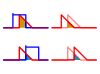
Figure 1: Construction of a partial covariance map of N₂ molecules undergoing Coulomb explosion induced by a free-electron laser.^[10] Panels a and b map the two terms of the covariance matrix, which is shown in panel c. Panel d maps common-mode correlations via intensity fluctuations of the laser. Panel e maps the partial covariance matrix that is corrected for the intensity fluctuations. Panel f shows that 10% overcorrection improves the map and makes ion-ion correlations clearly visible. Owing to momentum conservation these correlations appear as lines approximately perpendicular to the autocorrelation line (and to the periodic modulations which are caused by detector ringing).

Fig. 1 illustrates how a partial covariance map is constructed on an example of an experiment performed at the FLASH free-electron laser in Hamburg.^[10] The random function ${\displaystyle X(t)}$ is the time-of-flight spectrum of ions from a Coulomb explosion of nitrogen molecules multiply ionised by a laser pulse. Since only a few hundreds of molecules are ionised at each laser pulse, the single-shot spectra are highly fluctuating. However, collecting typically ${\displaystyle m=10^{4}}$ such spectra, ${\displaystyle \mathbf {X} _{j}(t)}$, and averaging them over ${\displaystyle j}$ produces a smooth spectrum ${\displaystyle \langle \mathbf {X} (t)\rangle }$, which is shown in red at the bottom of Fig. 1. The average spectrum ${\displaystyle \langle \mathbf {X} \rangle }$ reveals several nitrogen ions in a form of peaks broadened by their kinetic energy, but to find the correlations between the ionisation stages and the ion momenta requires calculating a covariance map.

In the example of Fig. 1 spectra ${\displaystyle \mathbf {X} _{j}(t)}$ and ${\displaystyle \mathbf {Y} _{j}(t)}$ are the same, except that the range of the time-of-flight ${\displaystyle t}$ differs. Panel a shows ${\displaystyle \langle \mathbf {XY^{\rm {T}}} \rangle }$, panel b shows ${\displaystyle \langle \mathbf {X} \rangle \langle \mathbf {Y^{\rm {T}}} \rangle }$ and panel c shows their difference, which is ${\displaystyle \operatorname {cov} (\mathbf {X} ,\mathbf {Y} )}$ (note a change in the colour scale). Unfortunately, this map is overwhelmed by uninteresting, common-mode correlations induced by laser intensity fluctuating from shot to shot. To suppress such correlations the laser intensity ${\displaystyle I_{j}}$ is recorded at every shot, put into ${\displaystyle \mathbf {I} }$ and ${\displaystyle \operatorname {pcov} (\mathbf {X} ,\mathbf {Y} \mid \mathbf {I} )}$ is calculated as panels d and e show. The suppression of the uninteresting correlations is, however, imperfect because there are other sources of common-mode fluctuations than the laser intensity and in principle all these sources should be monitored in vector ${\displaystyle \mathbf {I} }$. Yet in practice it is often sufficient to overcompensate the partial covariance correction as panel f shows, where interesting correlations of ion momenta are now clearly visible as straight lines centred on ionisation stages of atomic nitrogen.

Two-dimensional infrared spectroscopy[]

Two-dimensional infrared spectroscopy employs correlation analysis to obtain 2D spectra of the condensed phase. There are two versions of this analysis: synchronous and asynchronous. Mathematically, the former is expressed in terms of the sample covariance matrix and the technique is equivalent to covariance mapping.^[11]

See also[]

• Multivariate statistics
• Gramian matrix
• Eigenvalue decomposition
• Quadratic form (statistics)
• Principal components

References[]

Further reading[]

• "Covariance matrix", Encyclopedia of Mathematics, EMS Press, 2001 [1994]
• Weisstein, Eric W. "Covariance Matrix". MathWorld.
• van Kampen, N. G. (1981). Stochastic processes in physics and chemistry. New York: North-Holland. ISBN 0-444-86200-5.