Gompertz function

The Gompertz curve or Gompertz function is a type of mathematical model for a time series, named after Benjamin Gompertz (1779–1865). It is a sigmoid function which describes growth as being slowest at the start and end of a given time period. The right-hand or future value asymptote of the function is approached much more gradually by the curve than the left-hand or lower valued asymptote. This is in contrast to the simple logistic function in which both asymptotes are approached by the curve symmetrically. It is a special case of the generalised logistic function. The function was originally designed to describe human mortality, but since has been modified to be applied in biology, with regard to detailing populations.

History[]

Benjamin Gompertz (1779–1865) was an actuary in London who was privately educated.^[1] He was elected a fellow of the Royal Society in 1819. The function was first presented in his June 16, 1825 paper at the bottom of page 518.^[2] The Gompertz function reduced a significant collection of data in life tables into a single function. It is based on the assumption that the mortality rate increases exponentially as a person ages. The resulting Gompertz function is for the number of individuals living at a given age as a function of age.

Earlier work on the construction of functional models of mortality was done by the French mathematician Abraham de Moivre (1667–1754) in the 1750s.^[3][4] However, de Moivre assumed that the mortality rate was constant. An extension to Gompertz's work was proposed by the English actuary and mathematician William Matthew Makeham (1826–1891) in 1860, who added a constant background mortality rate to Gompertz’s exponentially increasing one.^[5]

Graphs of Gompertz curves, showing the effect of varying one of a,b,c while keeping the others constant

Varying ${\displaystyle a}$

Varying ${\displaystyle b}$

Varying ${\displaystyle c}$

Formula[]

where

• a is an asymptote, since ${\textstyle \lim _{t\to \infty }a\mathrm {e} ^{-\mathrm {e} ^{b-ct}}=a\mathrm {e} ^{0}=a}$
• b sets the displacement along the x-axis (translates the graph to the left or right).
• c sets the growth rate (y scaling)
• e is Euler's Number (e = 2.71828...)

Properties[]

The halfway point is found by solving ${\textstyle f(t)=a/2}$ for t.

The point of maximum rate of increase (${\textstyle 0.368a}$) is found by solving ${\textstyle {\frac {d^{2}}{dt^{2}}}f(t)=0}$ for t. The increase at ${\textstyle t_{max}}$ is

Derivation[]

The function curve can be derived from a Gompertz law of mortality, which states the rate of absolute mortality (decay) falls exponentially with current size. Mathematically,

where

• ${\textstyle r={\frac {y'(t)}{y(t)}}}$ is the rate of growth
• k is an arbitrary constant.

Example uses[]

Examples of uses for Gompertz curves include:

• Mobile phone uptake, where costs were initially high (so uptake was slow), followed by a period of rapid growth, followed by a slowing of uptake as saturation was reached^[6]
• Population in a confined space, as birth rates first increase and then slow as resource limits are reached^[7]
• Modelling of growth of tumors^[8]
• Modelling market impact in finance^[9] and aggregated subnational loans dynamic.^[10]
• Detailing population growth in animals of prey, with regard to predator-prey relationships
• Modelling bacterial cells within a population
• Examining disease spread

Applications[]

Gompertz curve[]

Population biology is especially concerned with the Gompertz function. This function is especially useful in describing the rapid growth of a certain population of organisms while also being able to account for the eventual horizontal asymptote, once the carrying capacity is determined (plateau cell/population number).

It is modeled as follows:

where:

• t is time
• N₀ is the initial amount of cells
• N_I is the plateau cell/population number
• b is the initial rate of tumor growth

This function consideration of the plateau cell number makes it useful in accurately mimicking real-life population dynamics. The function also adheres to the sigmoid function, which is the most widely accepted convention of generally detailing a population's growth. Moreover, the function makes use of initial growth rate, which is commonly seen in populations of bacterial and cancer cells, which undergo the log phase and grow rapidly in numbers. Despite its popularity, the function initial rate of tumor growth is difficult to predetermine given the varying microcosms present with a patient, or varying environmental factors in the case of population biology. In cancer patients, factors such as age, diet, ethnicity, genetic pre-dispositions, metabolism, lifestyle and origin of metastasis play a role in determining the tumor growth rate. The carrying capacity is also expected to change based on these factors, and so describing such phenomena is difficult.

Metabolic curve[]

The metabolic function is particularly concerned with accounting for the rate of metabolism within an organism. This function can be applied to monitor tumor cells; metabolic rate is dynamic and is greatly flexible, making it more precise in detailing cancer growth. The metabolic curve takes in to consideration the energy the body provides in maintaining and creating tissue. This energy can be considered as metabolism and follows a specific pattern in cellular division. Energy conservation can be used to model such growth, irrespective of differing masses and development times. All taxa share a similar growth pattern and this model, as a result, considers cellular division, the foundation of the development of a tumor.

• B = energy organism uses at rest
• N_C = number of cells in the given organism
• B_C= metabolic rate of an individual cell
• N_CB_C= energy required to maintain the existing tissue
• E_C= energy required to create new tissue from an individual cell

The differentiation between energy used at rest and metabolic rate work allows for the model to more precisely determine the rate of growth. The energy at rest is lower than the energy used to maintain a tissue, and together represent the energy required to maintain the existing tissue. The use of these two factors, alongside the energy required to create new tissue, comprehensively map the rate of growth, and moreover, lead in to an accurate representation of the lag phase.

Growth of tumors[]

In the 1960s A.K. Laird^[11] for the first time successfully used the Gompertz curve to fit data of growth of tumors. In fact, tumors are cellular populations growing in a confined space where the availability of nutrients is limited. Denoting the tumor size as X(t) it is useful to write the Gompertz Curve as follows:

${\displaystyle X(t)=K\exp \left(\log \left({\frac {X(0)}{K}}\right)\exp \left(-\alpha t\right)\right)}$

where:

• X(0) is the tumor size at the starting observation time;
• K is the carrying capacity, i.e. the maximum size that can be reached with the available nutrients. In fact it is:
  $${\displaystyle \lim _{t\rightarrow +\infty }X(t)=K}$$

  

independently on X(0)>0. Note that, in absence of therapies etc.. usually it is X(0) < K, whereas, in presence of therapies, it may be X(0) > K;

• α is a constant related to the proliferative ability of the cells.
• log() refers to the natural log.

It can be shown that the dynamics of X(t) are governed by the Gompertz differential equation:

i.e. is of the form when broken down:

F(X) is the instantaneous proliferation rate of the cellular population, whose decreasing nature is due to the competition for the nutrients due to the increase of the cellular population, similarly to the logistic growth rate. However, there is a fundamental difference: in the logistic case the proliferation rate for small cellular population is finite:

whereas in the Gompertz case the proliferation rate is unbounded:

As noticed by Steel^[12] and by Wheldon,^[13] the proliferation rate of the cellular population is ultimately bounded by the cell division time. Thus, this might be an evidence that the Gompertz equation is not good to model the growth of small tumors. Moreover, more recently it has been noticed^[14] that, including the interaction with immune system, Gompertz and other laws characterized by unbounded F(0) would preclude the possibility of immune surveillance.

The theoretical study by Fornalski et al. ^[15] showed the biophysical basis of the Gompertz curve for cancer growth except very early phase where parabolic function is more appropriate. They found also that the Gompertz curve describes the most typical case among the broad family of the cancer dynamics’ functions.

Gompertz growth and logistic growth[]

The Gompertz differential equation

is the limiting case of the generalized logistic differential equation

(where ${\displaystyle \nu >0}$ is a positive real number) since

.

In addition, there is an inflection point in the graph of the generalized logistic function when

and one in the graph of the Gompertz function when

.

Modeling COVID-19 infection trajectory[]

A generalized logistic function, also called the Richards growth curve, is widely used in modelling COVID-19 infection trajectories.^[16] Infection trajectory is a daily time series data for the cumulative number of infected cases for a subject such as country, city, state, etc. There are variant re-parameterizations in the literature: one of frequently used forms is

${\displaystyle f(t;\theta _{1},\theta _{2},\theta _{3},\xi )={\frac {\theta _{1}}{[1+\xi \exp(-\theta _{2}\cdot (t-\theta _{3}))]^{1/\xi }}}}$

where ${\displaystyle \theta _{1},\theta _{2},\theta _{3}}$ are real numbers, and ${\displaystyle \xi }$ is a positive real number. The flexibility of the curve ${\displaystyle f}$ is due to the parameter ${\displaystyle \xi }$: (i) if ${\displaystyle \xi =1}$ then the curve reduces to the logistic function, and (ii) if ${\displaystyle \xi }$ converges to zero, then the curve converges to the Gompertz function. In epidemiological modeling, ${\displaystyle \theta _{1}}$, ${\displaystyle \theta _{2}}$, and ${\displaystyle \theta _{3}}$ represent the final epidemic size, infection rate, and lag phase, respectively. See the right panel for an examplary infection trajectory when ${\displaystyle (\theta _{1},\theta _{2},\theta _{3})}$ are designated by ${\displaystyle (10,000,0.2,40)}$.

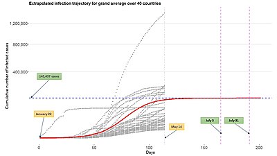
One of the benefits of using growth function such as generalized logistic function in epidemiological modeling is its relatively easy expansion to the multilevel model framework by using the growth function to describe infection trajectories from multiple subjects (countries, cities, states, etc). See the above figure. Such a modeling framework can be also widely called the nonlinear mixed-effects model or hierarchical nonlinear model.

Gomp-ex law of growth[]

Based on the above considerations, Wheldon^[13] proposed a mathematical model of tumor growth, called the Gomp-Ex model, that slightly modifies the Gompertz law. In the Gomp-Ex model it is assumed that initially there is no competition for resources, so that the cellular population expands following the exponential law. However, there is a critical size threshold ${\displaystyle X_{C}}$ such that for ${\displaystyle X>X_{C}}$. The assumption that there is no competition for resources holds true in most scenarios. It can however be affected by limiting factors, that requires the creation of sub-factors variables.

the growth follows the Gompertz Law:

so that:

Here there are some numerical estimates^[13] for ${\displaystyle X_{C}}$:

• ${\textstyle X_{C}\approx 10^{9}}$ for human tumors
• ${\textstyle X_{C}\approx 10^{6}}$ for murine (mouse) tumors

See also[]

• Gompertz distribution
• Growth curve
• Von Bertalanffy function
• Sigmoid function

References[]

External links[]

• Weisstein, Eric W. "Gompertz Curve". MathWorld.
• https://archive.org/details/philtrans04942340
• http://chemoth.com/tumorgrowth