Morse theory

In mathematics, specifically in differential topology, Morse theory enables one to analyze the topology of a manifold by studying differentiable functions on that manifold. According to the basic insights of Marston Morse, a typical differentiable function on a manifold will reflect the topology quite directly. Morse theory allows one to find CW structures and handle decompositions on manifolds and to obtain substantial information about their homology.

Before Morse, Arthur Cayley and James Clerk Maxwell had developed some of the ideas of Morse theory in the context of topography. Morse originally applied his theory to geodesics (critical points of the energy functional on paths). These techniques were used in Raoul Bott's proof of his periodicity theorem.

The analogue of Morse theory for complex manifolds is Picard–Lefschetz theory.

Basic concepts[]

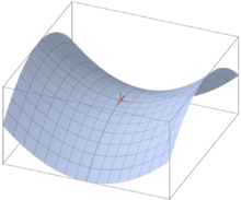
Consider, for purposes of illustration, a mountainous landscape ${\displaystyle M.}$ If ${\displaystyle f}$ is the function ${\displaystyle M\to \mathbb {R} }$ sending each point to its elevation, then the inverse image of a point in ${\displaystyle \mathbb {R} }$ is a contour line (more generally, a level set). Each connected component of a contour line is either a point, a simple closed curve, or a closed curve with a double point. Contour lines may also have points of higher order (triple points, etc.), but these are unstable and may be removed by a slight deformation of the landscape. Double points in contour lines occur at saddle points, or passes. Saddle points are points where the surrounding landscape curves up in one direction and down in the other.

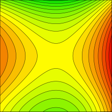
Imagine flooding this landscape with water. Then, the region covered by water when the water reaches an elevation of ${\displaystyle a}$ is ${\displaystyle f^{-1}(-\infty ,a]}$, or the points with elevation less than or equal to ${\displaystyle a.}$ Consider how the topology of this region changes as the water rises. It appears, intuitively, that it does not change except when ${\displaystyle a}$ passes the height of a critical point; that is, a point where the gradient of ${\displaystyle f}$ is ${\displaystyle 0}$ (that is the Jacobian matrix acting as a linear map from the tangent space at that point to the tangent space at its image under the map ${\displaystyle f}$ does not have maximal rank). In other words, it does not change except when the water either (1) starts filling a basin, (2) covers a saddle (a mountain pass), or (3) submerges a peak.

To each of these three types of critical points – basins, passes, and peaks (also called minima, saddles, and maxima) – one associates a number called the index. Intuitively speaking, the index of a critical point ${\displaystyle b}$ is the number of independent directions around ${\displaystyle b}$ in which ${\displaystyle f}$ decreases. More precisely the index of a non-degenerate critical point ${\displaystyle b}$ of ${\displaystyle f}$ is the dimension of the largest subspace of the tangent space to ${\displaystyle M}$ at ${\displaystyle b}$ on which the Hessian of ${\displaystyle f}$ is negative definite. Therefore, the indices of basins, passes, and peaks are ${\displaystyle 0,1,}$ and ${\displaystyle 2,}$ respectively.

Define ${\displaystyle M^{a}}$ as ${\displaystyle f^{-1}(-\infty ,a]}$. Leaving the context of topography, one can make a similar analysis of how the topology of ${\displaystyle M^{a}}$ changes as ${\displaystyle a}$ increases when ${\displaystyle M}$ is a torus oriented as in the image and ${\displaystyle f}$ is projection on a vertical axis, taking a point to its height above the plane.

Starting from the bottom of the torus, let ${\displaystyle p,q,r,}$ and ${\displaystyle s}$ be the four critical points of index ${\displaystyle 0,1,1,}$ and ${\displaystyle 2,}$ respectively. When ${\displaystyle a}$ is less than ${\displaystyle f(p)=0,}$ then ${\displaystyle M^{a}}$ is the empty set. After ${\displaystyle a}$ passes the level of ${\displaystyle p,}$ when ${\displaystyle 0<a<f(q),}$ then ${\displaystyle M^{a}}$ is a disk, which is homotopy equivalent to a point (a 0-cell), which has been "attached" to the empty set. Next, when ${\displaystyle a}$ exceeds the level of ${\displaystyle q,}$ and ${\displaystyle f(q)<a<f(r),}$ then ${\displaystyle M^{a}}$ is a cylinder, and is homotopy equivalent to a disk with a 1-cell attached (image at left). Once ${\displaystyle a}$ passes the level of ${\displaystyle r,}$ and ${\displaystyle f(r)<a<f(s),}$ then ${\displaystyle M^{1}}$ is a torus with a disk removed, which is homotopy equivalent to a cylinder with a 1-cell attached (image at right). Finally, when ${\displaystyle a}$ is greater than the critical level of ${\displaystyle s,}$ ${\displaystyle M^{a}}$ is a torus. A torus, of course, is the same as a torus with a disk removed with a disk (a 2-cell) attached.

One therefore appears to have the following rule: the topology of ${\displaystyle M^{\alpha }}$ does not change except when ${\displaystyle \alpha }$ passes the height of a critical point, and when ${\displaystyle \alpha }$ passes the height of a critical point of index ${\displaystyle \gamma }$, a ${\displaystyle \gamma }$-cell is attached to ${\displaystyle M^{\alpha }.}$ This does not address the question of what happens when two critical points are at the same height. That situation can be resolved by a slight perturbation of ${\displaystyle f.}$ In the case of a landscape (or a manifold embedded in Euclidean space), this perturbation might simply be tilting the landscape slightly, or rotating the coordinate system.

One should be careful and verify the non-degeneracy of critical points. To see what can pose a problem, let ${\displaystyle M=\mathbb {R} }$ and let ${\displaystyle f(x)=x^{3}.}$ Then ${\displaystyle 0}$ is a critical point of ${\displaystyle f,}$ but the topology of ${\displaystyle M^{\alpha }}$ does not change when ${\displaystyle \alpha }$ passes ${\displaystyle 0.}$ The problem is that the second derivative of ${\displaystyle f}$ is also ${\displaystyle 0}$ at ${\displaystyle 0,}$ that is, the Hessian of ${\displaystyle f}$ vanishes and this critical point is degenerate. Note that this situation is unstable: by slightly deforming ${\displaystyle f,}$ the degenerate critical point is either removed or breaks up into two non-degenerate critical points.

Formal development[]

For a real-valued smooth function ${\displaystyle f:M\to \mathbb {R} }$ on a differentiable manifold ${\displaystyle M,}$ the points where the differential of ${\displaystyle f}$ vanishes are called critical points of ${\displaystyle f}$ and their images under ${\displaystyle f}$ are called critical values. If at a critical point ${\displaystyle b,}$ the matrix of second partial derivatives (the Hessian matrix) is non-singular, then ${\displaystyle b}$ is called a non-degenerate critical point; if the Hessian is singular then ${\displaystyle b}$ is a degenerate critical point.

For the functions

from ${\displaystyle \mathbb {R} }$ to ${\displaystyle \mathbb {R} ,}$ ${\displaystyle f}$ has a critical point at the origin if ${\displaystyle b=0,}$ which is non-degenerate if ${\displaystyle c\neq 0}$ (that is, ${\displaystyle f}$ is of the form ${\displaystyle a+cx^{2}+\cdots }$) and degenerate if ${\displaystyle c=0}$ (that is, ${\displaystyle f}$ is of the form ${\displaystyle a+dx^{3}+\cdots }$). A less trivial example of a degenerate critical point is the origin of the monkey saddle.

The index of a non-degenerate critical point ${\displaystyle b}$ of ${\displaystyle f}$ is the dimension of the largest subspace of the tangent space to ${\displaystyle M}$ at ${\displaystyle b}$ on which the Hessian is negative definite. This corresponds to the intuitive notion that the index is the number of directions in which ${\displaystyle f}$ decreases. The degeneracy and index of a critical point are independent of the choice of the local coordinate system used, as shown by Sylvester's Law.

Morse lemma[]

Let ${\displaystyle b}$ be a non-degenerate critical point of ${\displaystyle f:M\to R.}$ Then there exists a chart ${\displaystyle \left(x_{1},x_{2},\ldots ,x_{n}\right)}$ in a neighborhood ${\displaystyle U}$ of ${\displaystyle b}$ such that ${\displaystyle x_{i}(b)=0}$ for all ${\displaystyle i}$ and

throughout ${\displaystyle U.}$ Here ${\displaystyle \alpha }$ is equal to the index of ${\displaystyle f}$ at ${\displaystyle b.}$ As a corollary of the Morse lemma, one sees that non-degenerate critical points are isolated. (Regarding an extension to the complex domain see Complex Morse Lemma. For a generalization, see Morse–Palais lemma).

Fundamental theorems[]

A smooth real-valued function on a manifold ${\displaystyle M}$ is a Morse function if it has no degenerate critical points. A basic result of Morse theory says that almost all functions are Morse functions. Technically, the Morse functions form an open, dense subset of all smooth functions ${\displaystyle M\to \mathbb {R} }$ in the ${\displaystyle C^{2}}$ topology. This is sometimes expressed as "a typical function is Morse" or "a generic function is Morse".

As indicated before, we are interested in the question of when the topology of ${\displaystyle M^{a}=f^{-1}(-\infty ,a]}$ changes as ${\displaystyle a}$ varies. Half of the answer to this question is given by the following theorem.

Theorem. Suppose ${\displaystyle f}$ is a smooth real-valued function on ${\displaystyle M,}$ ${\displaystyle a<b,}$ ${\displaystyle f^{-1}[a,b]}$ is compact, and there are no critical values between ${\displaystyle a}$ and ${\displaystyle b.}$ Then ${\displaystyle M^{a}}$ is diffeomorphic to ${\displaystyle M^{b},}$ and ${\displaystyle M^{b}}$ deformation retracts onto ${\displaystyle M^{a}.}$

It is also of interest to know how the topology of ${\displaystyle M^{a}}$ changes when ${\displaystyle a}$ passes a critical point. The following theorem answers that question.

Theorem. Suppose ${\displaystyle f}$ is a smooth real-valued function on ${\displaystyle M}$ and ${\displaystyle p}$ is a non-degenerate critical point of ${\displaystyle f}$ of index ${\displaystyle \gamma ,}$ and that ${\displaystyle f(p)=q.}$ Suppose ${\displaystyle f^{-1}[q-\varepsilon ,q+\varepsilon ]}$ is compact and contains no critical points besides ${\displaystyle p.}$ Then ${\displaystyle M^{q+\varepsilon }}$ is homotopy equivalent to ${\displaystyle M^{q-\varepsilon }}$ with a ${\displaystyle \gamma }$-cell attached.

These results generalize and formalize the 'rule' stated in the previous section.

Using the two previous results and the fact that there exists a Morse function on any differentiable manifold, one can prove that any differentiable manifold is a CW complex with an ${\displaystyle n}$-cell for each critical point of index ${\displaystyle n.}$ To do this, one needs the technical fact that one can arrange to have a single critical point on each critical level, which is usually proven by using gradient-like vector fields to rearrange the critical points.

Morse inequalities[]

Morse theory can be used to prove some strong results on the homology of manifolds. The number of critical points of index ${\displaystyle \gamma }$ of ${\displaystyle f:M\to \mathbb {R} }$ is equal to the number of ${\displaystyle \gamma }$ cells in the CW structure on ${\displaystyle M}$ obtained from "climbing" ${\displaystyle f.}$ Using the fact that the alternating sum of the ranks of the homology groups of a topological space is equal to the alternating sum of the ranks of the chain groups from which the homology is computed, then by using the cellular chain groups (see cellular homology) it is clear that the Euler characteristic ${\displaystyle \chi (M)}$ is equal to the sum

where ${\displaystyle C^{\gamma }}$ is the number of critical points of index ${\displaystyle \gamma .}$ Also by cellular homology, the rank of the ${\displaystyle n}$^th homology group of a CW complex ${\displaystyle M}$ is less than or equal to the number of ${\displaystyle n}$-cells in ${\displaystyle M.}$ Therefore, the rank of the ${\displaystyle \gamma }$^th homology group, that is, the Betti number ${\displaystyle b_{\gamma }(M)}$, is less than or equal to the number of critical points of index ${\displaystyle \gamma }$ of a Morse function on ${\displaystyle M.}$ These facts can be strengthened to obtain the Morse inequalities:

In particular, for any

one has

This gives a powerful tool to study manifold topology. Suppose on a closed manifold there exists a Morse function ${\displaystyle f:M\to \mathbb {R} }$ with precisely k critical points. In what way does the existence of the function ${\displaystyle f}$ restrict ${\displaystyle M}$? The case ${\displaystyle k=2}$ was studied by Georges Reeb in 1952; the Reeb sphere theorem states that ${\displaystyle M}$ is homeomorphic to a sphere ${\displaystyle S^{n}.}$ The case ${\displaystyle k=3}$ is possible only in a small number of low dimensions, and M is homeomorphic to an Eells–Kuiper manifold. In 1982 Edward Witten developed an analytic approach to the Morse inequalities by considering the de Rham complex for the perturbed operator ${\displaystyle d_{t}=e^{-tf}de^{tf}.}$^[1][2]

Application to classification of closed 2-manifolds[]

Morse theory has been used to classify closed 2-manifolds up to diffeomorphism. If ${\displaystyle M}$ is oriented, then ${\displaystyle M}$ is classified by its genus ${\displaystyle g}$ and is diffeomorphic to a sphere with ${\displaystyle g}$ handles: thus if ${\displaystyle g=0,}$ ${\displaystyle M}$ is diffeomorphic to the 2-sphere; and if ${\displaystyle g>0,}$ ${\displaystyle M}$ is diffeomorphic to the connected sum of ${\displaystyle g}$ 2-tori. If ${\displaystyle N}$ is unorientable, it is classified by a number ${\displaystyle g>0}$ and is diffeomorphic to the connected sum of ${\displaystyle g}$ real projective spaces ${\displaystyle \mathbf {RP} ^{2}.}$ In particular two closed 2-manifolds are homeomorphic if and only if they are diffeomorphic.^[3][4][5]

Morse homology[]

Morse homology is a particularly easy way to understand the homology of smooth manifolds. It is defined using a generic choice of Morse function and Riemannian metric. The basic theorem is that the resulting homology is an invariant of the manifold (that is,, independent of the function and metric) and isomorphic to the singular homology of the manifold; this implies that the Morse and singular Betti numbers agree and gives an immediate proof of the Morse inequalities. An infinite dimensional analog of Morse homology in symplectic geometry is known as Floer homology.

Morse–Bott theory[]

The notion of a Morse function can be generalized to consider functions that have nondegenerate manifolds of critical points. A Morse–Bott function is a smooth function on a manifold whose is a closed submanifold and whose Hessian is non-degenerate in the normal direction. (Equivalently, the kernel of the Hessian at a critical point equals the tangent space to the critical submanifold.) A Morse function is the special case where the critical manifolds are zero-dimensional (so the Hessian at critical points is non-degenerate in every direction, that is, has no kernel).

The index is most naturally thought of as a pair

where ${\displaystyle i_{-}}$ is the dimension of the unstable manifold at a given point of the critical manifold, and ${\displaystyle i_{+}}$ is equal to ${\displaystyle i_{-}}$ plus the dimension of the critical manifold. If the Morse–Bott function is perturbed by a small function on the critical locus, the index of all critical points of the perturbed function on a critical manifold of the unperturbed function will lie between ${\displaystyle i_{-}}$ and ${\displaystyle i_{+}.}$

Morse–Bott functions are useful because generic Morse functions are difficult to work with; the functions one can visualize, and with which one can easily calculate, typically have symmetries. They often lead to positive-dimensional critical manifolds. Raoul Bott used Morse–Bott theory in his original proof of the Bott periodicity theorem.

Round functions are examples of Morse–Bott functions, where the critical sets are (disjoint unions of) circles.

Morse homology can also be formulated for Morse–Bott functions; the differential in Morse–Bott homology is computed by a spectral sequence. Frederic Bourgeois sketched an approach in the course of his work on a Morse–Bott version of symplectic field theory, but this work was never published due to substantial analytic difficulties.

See also[]

References[]

Further reading[]

• Bott, Raoul (1988). "Morse Theory Indomitable". Publications Mathématiques de l'IHÉS. 68: 99–114. doi:10.1007/bf02698544.
• Bott, Raoul (1982). "Lectures on Morse theory, old and new". Bulletin of the American Mathematical Society. (N.S.). 7 (2): 331–358. doi:10.1090/s0273-0979-1982-15038-8.
• Cayley, Arthur (1859). "On Contour and Slope Lines" (PDF). The Philosophical Magazine. 18 (120): 264–268.
• Guest, Martin (2001). "Morse Theory in the 1990s". arXiv:math/0104155. Cite journal requires |journal= (help)
• Hirsch, M. (1994). Differential Topology (2nd ed.). Springer.
• (19 October 2007). Differential Manifolds. Dover Book on Mathematics (Reprint of 1993 ed.). Mineola, New York: Dover Publications. ISBN 978-0-486-46244-8. OCLC 853621933.
• Lang, Serge (1999). Fundamentals of Differential Geometry. Graduate Texts in Mathematics. 191. New York: Springer-Verlag. ISBN 978-0-387-98593-0. OCLC 39379395.
• Matsumoto, Yukio (2002). An Introduction to Morse Theory.
• Maxwell, James Clerk (1870). "On Hills and Dales" (PDF). The Philosophical Magazine. 40 (269): 421–427.
• Milnor, John (1963). Morse Theory. Princeton University Press. ISBN 0-691-08008-9. A classic advanced reference in mathematics and mathematical physics.
• Milnor, John (1965). Lectures on the h-cobordism theorem (PDF).
• Morse, Marston (1934). The Calculus of Variations in the Large. American Mathematical Society Colloquium Publication. 18. New York.
• Schwarz, Matthias (1993). Morse Homology. Birkhäuser.