Matrices important in quantum mechanics and the study of spin
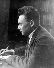
Wolfgang Pauli (1900–1958), ca. 1924. Pauli received the Nobel Prize in physics in 1945, nominated by Albert Einstein, for the Pauli exclusion principle.
These matrices are named after the physicist Wolfgang Pauli. In quantum mechanics, they occur in the Pauli equation which takes into account the interaction of the spin of a particle with an external electromagnetic field.
Each Pauli matrix is Hermitian, and together with the identity matrix I (sometimes considered as the zeroth Pauli matrix σ0), the Pauli matrices form a basis for the real vector space of 2 × 2 Hermitian matrices.
This means that any 2 × 2Hermitian matrix can be written in a unique way as a linear combination of Pauli matrices, with all coefficients being real numbers.
Hermitian operators represent observables in quantum mechanics, so the Pauli matrices span the space of observables of the complex2-dimensional Hilbert space. In the context of Pauli's work, σk represents the observable corresponding to spin along the kth coordinate axis in three-dimensional Euclidean space
The Pauli matrices (after multiplication by i to make them anti-Hermitian) also generate transformations in the sense of Lie algebras: the matrices iσ1, iσ2, iσ3 form a basis for the real Lie algebra , which exponentiates to the special unitary group SU(2).[a] The algebra generated by the three matrices σ1, σ2, σ3 is isomorphic to the Clifford algebra of [citation needed], and the (unital associative) algebra generated by iσ1, iσ2, iσ3 is effectively identical (isomorphic) to that of quaternions ().
All three of the Pauli matrices can be compacted into a single expression:
where i = √−1 is the "imaginary unit", and δjk is the Kronecker delta, which equals +1 if j = k and 0 otherwise. This expression is useful for "selecting" any one of the matrices numerically by substituting values of j = 1, 2, 3, in turn useful when any of the matrices (but no particular one) is to be used in algebraic manipulations.
The determinants and traces of the Pauli matrices are:
From which, we can deduce that each matrix σjk has eigenvalues +1 and −1 .
With the inclusion of the identity matrix, I (sometimes denoted σ0), the Pauli matrices form an orthogonal basis (in the sense of Hilbert–Schmidt) of the Hilbert space of real2 × 2 Hermitian matrices, , and the Hilbert space of all complex2 × 2 matrices, .
Eigenvectors and eigenvalues[]
Each of the (Hermitian) Pauli matrices has two eigenvalues, +1 and −1. The corresponding normalizedeigenvectors are:
The Pauli matrices obey the following commutation relations:
and anticommutation relations:
where the structure constantεabc is the Levi-Civita symbol, Einstein summation notation is used, δjk is the Kronecker delta, and I is the 2 × 2 identity matrix.
For example,
commutators
anticommutators
Relation to dot and cross product[]
Pauli vectors elegantly map these commutation and anticommutation relations to corresponding vector products. Adding the commutator to the anticommutator gives
so that,
Contracting each side of the equation with components of two 3-vectors ap and bq (which commute with the Pauli matrices, i.e., apσq = σqap) for each matrix σq and vector component ap (and likewise with bq) yields
Finally, translating the index notation for the dot product and cross product results in
(1)
If i is identified with the pseudoscalar σxσyσz then the right hand side becomes which is also the definition for the product of two vectors in geometric algebra.
Some trace relations[]
The following traces can be derived using the commutation and anticommutation relations.
If the matrix σ0 = I is also considered, these relationships become
where Greek indices α, β, γ and μ assume values from {0, x, y, z} and the notation is used to denote the sum over the cyclic permutation of the included indices.
Exponential of a Pauli vector[]
For
one has, for even powers, 2p, p = 0, 1, 2, 3, ...
which can be shown first for the p = 1 case using the anticommutation relations. For convenience, the case p = 0 is taken to be I by convention.
In the last line, the first sum is the cosine, while the second sum is the sine; so, finally,
(2)
which is analogous to Euler's formula, extended to quaternions.
Note that
,
while the determinant of the exponential itself is just 1, which makes it the generic group element of SU(2).
A more abstract version of formula (2) for a general 2 × 2 matrix can be found in the article on matrix exponentials. A general version of (2) for an analytic (at a and −a) function is provided by application of Sylvester's formula,[3]
The group composition law of SU(2)[]
A straightforward application of formula (2) provides a parameterization of the composition law of the group SU(2).[c] One may directly solve for c in
which specifies the generic group multiplication, where, manifestly,
An alternative notation that is commonly used for the Pauli matrices is to write the vector index k in the superscript, and the matrix indices as subscripts, so that the element in row α and column β of the k-th Pauli matrix is σ kαβ .
In this notation, the completeness relation for the Pauli matrices can be written
Proof: The fact that the Pauli matrices, along with the identity matrix I, form an orthogonal basis for the Hilbert space of all 2 × 2 complex matrices means that we can express any matrix M as
where c is a complex number, and a is a 3 component, complex vector. It is straightforward to show, using the properties listed above, that
As noted above, it is common to denote the 2 × 2 unit matrix by σ0, so σ0αβ = δαβ . The completeness relation can alternatively be expressed as
The fact that any Hermitian complex 2 × 2 matrices can be expressed in terms of the identity matrix and the Pauli matrices also leads to the Bloch sphere representation of 2 × 2 mixed states’ density matrix, (positive semidefinite 2 × 2 matrices with unit trace. This can be seen by first expressing an arbitrary Hermitian matrix as a real linear combination of { σ0, σ1, σ2, σ3 } as above, and then imposing the positive-semidefinite and trace1 conditions.
For a pure state, in polar coordinates,
, the idempotent density matrix
acts on the state eigenvector with eigenvalue +1, hence it acts like a projection operator.
Relation with the permutation operator[]
Let Pjk be the transposition (also known as a permutation) between two spins σj and σk living in the tensor product space ,
This operator can also be written more explicitly as Dirac's spin exchange operator,
Its eigenvalues are therefore[d] 1 or −1. It may thus be utilized as an interaction term in a Hamiltonian, splitting the energy eigenvalues of its symmetric versus antisymmetric eigenstates.
SU(2)[]
The group SU(2) is the Lie group of unitary2 × 2 matrices with unit determinant; its Lie algebra is the set of all 2 × 2 anti-Hermitian matrices with trace 0. Direct calculation, as above, shows that the Lie algebra is the 3-dimensional real algebra spanned by the set {iσk}. In compact notation,
As a result, each i σj can be seen as an infinitesimal generator of SU(2). The elements of SU(2) are exponentials of linear combinations of these three generators, and multiply as indicated above in discussing the Pauli vector. Although this suffices to generate SU(2), it is not a proper representation of su(2), as the Pauli eigenvalues are scaled unconventionally. The conventional normalization is λ = 1/2, so that
The Lie algebra su(2) is isomorphic to the Lie algebra so(3), which corresponds to the Lie group SO(3), the group of rotations in three-dimensional space. In other words, one can say that the i σj are a realization (and, in fact, the lowest-dimensional realization) of infinitesimal rotations in three-dimensional space. However, even though su(2) and so(3) are isomorphic as Lie algebras, SU(2) and SO(3) are not isomorphic as Lie groups. SU(2) is actually a double cover of SO(3), meaning that there is a two-to-one group homomorphism from SU(2) to SO(3), see relationship between SO(3) and SU(2).
Quaternions[]
Main article: Spinor § Three dimensions
The real linear span of { I, i σ1, i σ2, i σ3 } is isomorphic to the real algebra of quaternions, represented by the span of the basis vectors The isomorphism from to this set is given by the following map (notice the reversed signs for the Pauli matrices):
Alternatively, the isomorphism can be achieved by a map using the Pauli matrices in reversed order,[5]
As the set of versorsU ⊂ forms a group isomorphic to SU(2), U gives yet another way of describing SU(2). The two-to-one homomorphism from SU(2) to SO(3) may be given in terms of the Pauli matrices in this formulation.
In classical mechanics, Pauli matrices are useful in the context of the Cayley-Klein parameters.[6] The matrix P corresponding to the position of a point in space is defined in terms of the above Pauli vector matrix,
Consequently, the transformation matrix Qθ for rotations about the x-axis through an angle θ may be written in terms of Pauli matrices and the unit matrix as[6]
Similar expressions follow for general Pauli vector rotations as detailed above.
Quantum mechanics[]
In quantum mechanics, each Pauli matrix is related to an angular momentum operator that corresponds to an observable describing the spin of a spin 1⁄2 particle, in each of the three spatial directions. As an immediate consequence of the Cartan decomposition mentioned above, iσj are the generators of a projective representation (spin representation) of the rotation group SO(3) acting on non-relativistic particles with spin 1⁄2. The states of the particles are represented as two-component spinors. In the same way, the Pauli matrices are related to the isospin operator.
An interesting property of spin 1⁄2 particles is that they must be rotated by an angle of 4π in order to return to their original configuration. This is due to the two-to-one correspondence between SU(2) and SO(3) mentioned above, and the fact that, although one visualizes spin up/down as the north/south pole on the 2-sphereS2, they are actually represented by orthogonal vectors in the two dimensional complex Hilbert space.
For a spin 1⁄2 particle, the spin operator is given by J = ħ/2σ, the fundamental representation of SU(2). By taking Kronecker products of this representation with itself repeatedly, one may construct all higher irreducible representations. That is, the resulting spin operators for higher spin systems in three spatial dimensions, for arbitrarily large j, can be calculated using this spin operator and ladder operators. They can be found in Rotation group SO(3)#A note on Lie algebra. The analog formula to the above generalization of Euler's formula for Pauli matrices, the group element in terms of spin matrices, is tractable, but less simple.[7]
Also useful in the quantum mechanics of multiparticle systems, the general Pauli groupGn is defined to consist of all n-fold tensor products of Pauli matrices.
Relativistic quantum mechanics[]
In relativistic quantum mechanics, the spinors in four dimensions are 4 × 1 (or 1 × 4) matrices. Hence the Pauli matrices or the Sigma matrices operating on these spinors have to be 4 × 4 matrices. They are defined in terms of 2 × 2 Pauli matrices as
It follows from this definition that the matrices have the same algebraic properties as the σk matrices.
However, relativistic angular momentum is not a three-vector, but a second order four-tensor. Hence needs to be replaced by Σμν, the generator of Lorentz transformations on spinors. By the antisymmetry of angular momentum, the Σμν are also antisymmetric. Hence there are only six independent matrices.
The first three are the The remaining three, where the Dirac αk matrices are defined as
The relativistic spin matrices Σμν are written in compact form in terms of commutator of gamma matrices as
Quantum information[]
In quantum information, single-qubitquantum gates are 2 × 2 unitary matrices. The Pauli matrices are some of the most important single-qubit operations. In that context, the Cartan decomposition given above is called the "Z–Y decomposition of a single-qubit gate". Choosing a different Cartan pair gives a similar "X–Y decomposition of a single-qubit gate".
For higher spin generalizations of the Pauli matrices, see spin (physics) § Higher spins
Exchange matrix (the second Pauli matrix is an exchange matrix of order two)
Remarks[]
^
This conforms to the convention in mathematics for the matrix exponential, iσ ↦ exp(iσ). In the convention in physics, σ ↦ exp(−iσ), hence in it no pre-multiplication by i is necessary to land in SU(2).
^
The Pauli vector is a formal device. It may be thought of as an element of ℳ2() ⊗ , where the tensor product space is endowed with a mapping ⋅ : × (ℳ2() ⊗ ) → ℳ2() induced by the dot product on
^The relation among a, b, c, n, m, k derived here in the 2 × 2 representation holds for all representations of SU(2), being a group identity. Note that, by virtue of the standard normalization of that group's generators as half the Pauli matrices, the parameters a,b,c correspond to half the rotation angles of the rotation group.
^
Explicitly, in the convention of "right-space matrices into elements of left-space matrices", it is
Notes[]
^"Pauli matrices". Planetmath website. 28 March 2008. Retrieved 28 May 2013.
^Nielsen, Michael A.; Chuang, Isaac L. (2000). Quantum Computation and Quantum Information. Cambridge, UK: Cambridge University Press. ISBN978-0-521-63235-5. OCLC43641333.


![{\displaystyle [\sigma _{j},\sigma _{k}]=2i\varepsilon _{jk\ell }\,\sigma _{\ell }~,}](https://wikimedia.org/api/rest_v1/media/math/render/svg/4f4d87176aff632a8f18b02c390f5b7a82271bb5)

![{\displaystyle {\begin{aligned}\left[\sigma _{1},\sigma _{2}\right]&=2i\sigma _{3}\\\left[\sigma _{2},\sigma _{3}\right]&=2i\sigma _{1}\\\left[\sigma _{3},\sigma _{1}\right]&=2i\sigma _{2}\\\left[\sigma _{1},\sigma _{1}\right]&=0\end{aligned}}}](https://wikimedia.org/api/rest_v1/media/math/render/svg/1d17d061cc37f2faf273f71466d73953c5cf995f)

![{\displaystyle {\begin{aligned}\left[\sigma _{j},\sigma _{k}\right]+\{\sigma _{j},\sigma _{k}\}&=(\sigma _{j}\sigma _{k}-\sigma _{k}\sigma _{j})+(\sigma _{j}\sigma _{k}+\sigma _{k}\sigma _{j})\\2i\varepsilon _{jk\ell }\,\sigma _{\ell }+2\delta _{jk}I&=2\sigma _{j}\sigma _{k}\end{aligned}}}](https://wikimedia.org/api/rest_v1/media/math/render/svg/610aa4fbda5736e477bd004340dee1c6e95fac5c)


![{\displaystyle {\begin{aligned}e^{ia\left({\hat {n}}\cdot {\vec {\sigma }}\right)}&=\sum _{k=0}^{\infty }{\frac {i^{k}\left[a\left({\hat {n}}\cdot {\vec {\sigma }}\right)\right]^{k}}{k!}}\\&=\sum _{p=0}^{\infty }{\frac {(-1)^{p}(a{\hat {n}}\cdot {\vec {\sigma }})^{2p}}{(2p)!}}+i\sum _{q=0}^{\infty }{\frac {(-1)^{q}(a{\hat {n}}\cdot {\vec {\sigma }})^{2q+1}}{(2q+1)!}}\\&=I\sum _{p=0}^{\infty }{\frac {(-1)^{p}a^{2p}}{(2p)!}}+i({\hat {n}}\cdot {\vec {\sigma }})\sum _{q=0}^{\infty }{\frac {(-1)^{q}a^{2q+1}}{(2q+1)!}}\\\end{aligned}}}](https://wikimedia.org/api/rest_v1/media/math/render/svg/d72e640e54da92d32160753e65de29076aaf8b3c)

![\det[i a(\hat{n} \cdot \vec{\sigma})] = a^2](https://wikimedia.org/api/rest_v1/media/math/render/svg/6101197de6277f0051a565f637da03e4068d40b8)


![{\displaystyle {\begin{aligned}c&={\tfrac {1}{2}}\,\operatorname {tr} \,M\,,\quad \ a_{k}={\tfrac {1}{2}}\,\operatorname {tr} \,\sigma ^{k}\,M~.\\[3pt]\therefore ~~2\,M&=I\,\operatorname {tr} \,M+\sum _{k}\sigma ^{k}\,\operatorname {tr} \,\sigma ^{k}M~,\end{aligned}}}](https://wikimedia.org/api/rest_v1/media/math/render/svg/424d48435c496789549e1c28a48eb1edc9b7919a)


![{\displaystyle \Sigma _{\mu \nu }={\frac {i}{2}}\left[\gamma _{\mu },\gamma _{\nu }\right]~.}](https://wikimedia.org/api/rest_v1/media/math/render/svg/27fea0fdeddef60669e2cce44ffc9f4072858231)

