Weierstrass substitution

In integral calculus, the Weierstrass substitution or tangent half-angle substitution is a method for evaluating integrals, which converts a rational function of trigonometric functions of ${\displaystyle x}$ into an ordinary rational function of ${\displaystyle t}$ by setting ${\displaystyle t=\tan(x/2)}$.^[1][2] No generality is lost by taking these to be rational functions of the sine and cosine. The general transformation formula is

${\displaystyle \int f(\sin(x),\cos(x))\,dx=\int f\left({\frac {2t}{1+t^{2}}},{\frac {1-t^{2}}{1+t^{2}}}\right){\frac {2\,dt}{1+t^{2}}}.}$

It is named after Karl Weierstrass (1815–1897),^[3][4][5] though it can be found in a book by Leonhard Euler from 1768.^[6] Michael Spivak wrote that this method was the "sneakiest substitution" in the world.^[7]

The substitution[]

Starting with a rational function of sines and cosines, one replaces ${\displaystyle \sin x}$ and ${\displaystyle \cos x}$ with rational functions of the variable ${\displaystyle t}$ and relates the differentials ${\displaystyle dx}$ and ${\displaystyle dt}$ as follows.

Let ${\displaystyle t=\tan(x/2)}$, where ${\displaystyle -\pi <x<\pi }$. Then^[1][8]

${\displaystyle \sin \left({\frac {x}{2}}\right)={\frac {t}{\sqrt {1+t^{2}}}}\qquad {\text{and}}\qquad \cos \left({\frac {x}{2}}\right)={\frac {1}{\sqrt {1+t^{2}}}}.}$

Hence,

${\displaystyle \sin x={\frac {2t}{1+t^{2}}},\qquad \cos x={\frac {1-t^{2}}{1+t^{2}}},\qquad {\text{and}}\qquad dx={\frac {2}{1+t^{2}}}\,dt.}$

Derivation of the formulas[]

By the double-angle formulas,

${\displaystyle \sin x=2\sin \left({\frac {x}{2}}\right)\cos \left({\frac {x}{2}}\right)=2\cdot {\frac {t}{\sqrt {t^{2}+1}}}\cdot {\frac {1}{\sqrt {t^{2}+1}}}={\frac {2t}{t^{2}+1}},}$

and

${\displaystyle \cos x=2\cos ^{2}\left({\frac {x}{2}}\right)-1={\frac {2}{t^{2}+1}}-1={\frac {2-(t^{2}+1)}{t^{2}+1}}={\frac {1-t^{2}}{1+t^{2}}}.}$

Finally, since ${\displaystyle t=\tan \left({\frac {x}{2}}\right)}$,

${\displaystyle dt={\frac {1}{2}}\sec ^{2}\left({\frac {x}{2}}\right)dx={\frac {dx}{2\cos ^{2}{\frac {x}{2}}}}={\frac {dx}{2\cdot {\frac {1}{t^{2}+1}}}}\qquad \Rightarrow \qquad dx={\frac {2}{t^{2}+1}}dt.}$

Examples[]

First example: the cosecant integral[]

${\displaystyle {\begin{aligned}\int \csc x\,dx&=\int {\frac {dx}{\sin x}}\\[6pt]&=\int \left({\frac {1+t^{2}}{2t}}\right)\left({\frac {2}{1+t^{2}}}\right)dt&&t=\tan {\frac {x}{2}}\\[6pt]&=\int {\frac {dt}{t}}\\[6pt]&=\ln |t|+C\\[6pt]&=\ln \left|\tan {\frac {x}{2}}\right|+C.\end{aligned}}}$

We can confirm the above result using a standard method of evaluating the cosecant integral by multiplying the numerator and denominator by ${\displaystyle \csc x-\cot x}$ and performing the following substitutions to the resulting expression: ${\displaystyle u=\csc x-\cot x}$ and ${\displaystyle du=(-\csc x\cot x+\csc ^{2}x)\,dx}$. This substitution can be obtained from the difference of the derivatives of cosecant and cotangent, which have cosecant as a common factor.

${\displaystyle {\begin{aligned}\int \csc x\,dx&=\int {\frac {\csc x(\csc x-\cot x)}{\csc x-\cot x}}\,dx\\[6pt]&=\int {\frac {(\csc ^{2}x-\csc x\cot x)\,dx}{\csc x-\cot x}}&&u=\csc x-\cot x\\[6pt]&=\int {\frac {du}{u}}&&du=(-\csc x\cot x+\csc ^{2}x)\,dx\\[6pt]&=\ln |u|+C=\ln |\csc x-\cot x|+C.\end{aligned}}}$

Now, the half-angle formulas for sines and cosines are

${\displaystyle \sin ^{2}\theta ={\frac {1-\cos 2\theta }{2}}\quad {\text{and}}\quad \cos ^{2}\theta ={\frac {1+\cos 2\theta }{2}}.}$

They give

${\displaystyle {\begin{aligned}\int \csc x\,dx&=\ln \left|\tan {\frac {x}{2}}\right|+C=\ln {\sqrt {\frac {1-\cos x}{1+\cos x}}}+C\\[6pt]&=\ln {\sqrt {{\frac {1-\cos x}{1+\cos x}}\cdot {\frac {1-\cos x}{1-\cos x}}}}+C\\[6pt]&=\ln {\sqrt {\frac {(1-\cos x)^{2}}{\sin ^{2}x}}}+C\\[6pt]&=\ln {\sqrt {\left({\frac {1-\cos x}{\sin x}}\right)^{2}}}+C\\[6pt]&=\ln {\sqrt {\left({\frac {1}{\sin x}}-{\frac {\cos x}{\sin x}}\right)^{2}}}+C\\[6pt]&=\ln {\sqrt {(\csc x-\cot x)^{2}}}+C=\ln \left|\csc x-\cot x\right|+C,\end{aligned}}}$

so the two answers are equivalent. The expression

${\displaystyle \tan {\frac {x}{2}}={\frac {1-\cos x}{\sin x}}}$

is a tangent half-angle formula. The secant integral may be evaluated in a similar manner.

Second example: a definite integral[]

${\displaystyle {\begin{aligned}\int _{0}^{2\pi }{\frac {dx}{2+\cos x}}&=\int _{0}^{\pi }{\frac {dx}{2+\cos x}}+\int _{\pi }^{2\pi }{\frac {dx}{2+\cos x}}\\[6pt]&=\int _{0}^{\infty }{\frac {2\,dt}{3+t^{2}}}+\int _{-\infty }^{0}{\frac {2\,dt}{3+t^{2}}}&t&=\tan {\frac {x}{2}}\\[6pt]&=\int _{-\infty }^{\infty }{\frac {2\,dt}{3+t^{2}}}\\[6pt]&={\frac {2}{\sqrt {3}}}\int _{-\infty }^{\infty }{\frac {du}{1+u^{2}}}&t&=u{\sqrt {3}}\\[6pt]&={\frac {2\pi }{\sqrt {3}}}.\end{aligned}}}$

In the first line, one does not simply substitute ${\displaystyle t=0}$ for both limits of integration. The singularity (in this case, a vertical asymptote) of ${\displaystyle t=\tan {\frac {x}{2}}}$ at ${\displaystyle x=\pi }$ must be taken into account. Alternatively, first evaluate the indefinite integral then apply the boundary values.

${\displaystyle {\begin{aligned}\int {\frac {dx}{2+\cos x}}&=\int {\frac {1}{2+{\frac {1-t^{2}}{1+t^{2}}}}}{\frac {2\,dt}{t^{2}+1}}&&t=\tan {\frac {x}{2}}\\[6pt]&=\int {\frac {2\,dt}{2(t^{2}+1)+(1-t^{2})}}=\int {\frac {2\,dt}{t^{2}+3}}\\[6pt]&={\frac {2}{3}}\int {\frac {dt}{\left({\frac {t}{\sqrt {3}}}\right)^{2}+1}}&&u={\frac {t}{\sqrt {3}}}\\[6pt]&={\frac {2}{\sqrt {3}}}\int {\frac {du}{u^{2}+1}}&&\tan \theta =u\\[6pt]&={\frac {2}{\sqrt {3}}}\int \cos ^{2}\theta \sec ^{2}\theta \,d\theta ={\frac {2}{\sqrt {3}}}\int d\theta \\[6pt]&={\frac {2}{\sqrt {3}}}\theta +C={\frac {2}{\sqrt {3}}}\arctan \left({\frac {t}{\sqrt {3}}}\right)+C\\[6pt]&={\frac {2}{\sqrt {3}}}\arctan \left[{\frac {\tan(x/2)}{\sqrt {3}}}\right]+C.\end{aligned}}}$

By symmetry,

${\displaystyle {\begin{aligned}\int _{0}^{2\pi }{\frac {dx}{2+\cos x}}&=2\int _{0}^{\pi }{\frac {dx}{2+\cos x}}=\lim _{b\rightarrow \pi }{\frac {4}{\sqrt {3}}}\arctan \left({\frac {\tan x/2}{\sqrt {3}}}\right){\Biggl |}_{0}^{b}\\[6pt]&={\frac {4}{\sqrt {3}}}{\Biggl [}\lim _{b\rightarrow \pi }\arctan \left({\frac {\tan b/2}{\sqrt {3}}}\right)-\arctan(0){\Biggl ]}={\frac {4}{\sqrt {3}}}\left({\frac {\pi }{2}}-0\right)={\frac {2\pi }{\sqrt {3}}},\end{aligned}}}$

which is the same as the previous answer.

Third example: both sine and cosine[]

${\displaystyle {\begin{aligned}\int {\frac {dx}{a\cos x+b\sin x+c}}&=\int {\frac {2dt}{a(1-t^{2})+2bt+c(t^{2}+1)}}\\[6pt]&=\int {\frac {2dt}{(c-a)t^{2}+2bt+a+c}}\\[6pt]&={\frac {2}{\sqrt {c^{2}-(a^{2}+b^{2})}}}\arctan {\frac {(c-a)\tan {\frac {x}{2}}+b}{\sqrt {c^{2}-(a^{2}+b^{2})}}}+C\end{aligned}}}$

If ${\displaystyle 4E=4(c-a)(c+a)-(2b)^{2}=4(c^{2}-(a^{2}+b^{2}))>0.}$

Geometry[]

The Weierstrass substitution parametrizes the unit circle centered at (0, 0). Instead of +∞ and −∞, we have only one ∞, at both ends of the real line. That is often appropriate when dealing with rational functions and with trigonometric functions. (This is the one-point compactification of the line.)

As x varies, the point (cos x, sin x) winds repeatedly around the unit circle centered at (0, 0). The point

${\displaystyle \left({\frac {1-t^{2}}{1+t^{2}}},{\frac {2t}{1+t^{2}}}\right)}$

goes only once around the circle as t goes from −∞ to +∞, and never reaches the point (−1, 0), which is approached as a limit as t approaches ±∞. As t goes from −∞ to −1, the point determined by t goes through the part of the circle in the third quadrant, from (−1, 0) to (0, −1). As t goes from −1 to 0, the point follows the part of the circle in the fourth quadrant from (0, −1) to (1, 0). As t goes from 0 to 1, the point follows the part of the circle in the first quadrant from (1, 0) to (0, 1). Finally, as t goes from 1 to +∞, the point follows the part of the circle in the second quadrant from (0, 1) to (−1, 0).

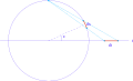
Here is another geometric point of view. Draw the unit circle, and let P be the point (−1, 0). A line through P (except the vertical line) is determined by its slope. Furthermore, each of the lines (except the vertical line) intersects the unit circle in exactly two points, one of which is P. This determines a function from points on the unit circle to slopes. The trigonometric functions determine a function from angles to points on the unit circle, and by combining these two functions we have a function from angles to slopes.

Gallery[]

• 

  (1/2) The Weierstrass substitution relates an angle to the slope of a line.

• 

  (2/2) The Weierstrass substitution illustrated as stereographic projection of the circle.

Hyperbolic functions[]

As with other properties shared between the trigonometric functions and the hyperbolic functions, it is possible to use hyperbolic identities to construct a similar form of the substitution:

${\displaystyle {\begin{aligned}&\sinh x={\frac {2t}{1-t^{2}}},\qquad \cosh x={\frac {1+t^{2}}{1-t^{2}}},\qquad \tanh x={\frac {2t}{1+t^{2}}},\\[6pt]&\coth x={\frac {1+t^{2}}{2t}},\qquad \operatorname {sech} x={\frac {1-t^{2}}{1+t^{2}}},\qquad \operatorname {csch} x={\frac {1-t^{2}}{2t}},\\[6pt]&{\text{and}}\qquad dx={\frac {2}{1-t^{2}}}\,dt.\end{aligned}}}$

See also[]

• Rational curve
• Stereographic projection
• Tangent half-angle formula
• Trigonometric substitution
• Euler substitution

Further reading[]

• Edwards, Joseph (1921). "Chapter VI". A Treatise on the Integral Calculus with Applications, Examples, and Problems. London: Macmillan and Co, Ltd.

Notes and references[]

External links[]

• Weierstrass substitution formulas at PlanetMath