Backward induction
Backward induction is the process of reasoning backwards in time, from the end of a problem or situation, to determine a sequence of optimal actions. It proceeds by examining the last point at which a decision is to be made and then identifying what action would be most optimal at that moment. Using this information, one can then determine what to do at the second-to-last time of decision. This process continues backwards until one has determined the best action for every possible situation (i.e. for every possible information set) at every point in time. Backward induction was first used in 1875 by Arthur Cayley, who uncovered the method while trying to solve the infamous Secretary problem.[1]
In the mathematical optimization method of dynamic programming, backward induction is one of the main methods for solving the Bellman equation.[2][3] In game theory, backward induction is a method used to compute subgame perfect equilibria in sequential games.[4] The only difference is that optimization involves just one decision maker, who chooses what to do at each point of time, whereas game theory analyzes how the decisions of several players interact. That is, by anticipating what the last player will do in each situation, it is possible to determine what the second-to-last player will do, and so on. In the related fields of automated planning and scheduling and automated theorem proving, the method is called backward search or backward chaining. In chess it is called retrograde analysis.
Backward induction has been used to solve games as long as the field of game theory has existed. John von Neumann and Oskar Morgenstern suggested solving zero-sum, two-person games by backward induction in their Theory of Games and Economic Behavior (1944), the book which established game theory as a field of study.[5][6]
Backward induction in decision making: an optimal-stopping problem[]
Consider an unemployed person who will be able to work for ten more years t = 1,2,...,10. Suppose that each year in which they remain unemployed, they may be offered a 'good' job that pays $100, or a 'bad' job that pays $44, with equal probability (50/50). Once they accept a job, they will remain in that job for the rest of the ten years. (Assume for simplicity that they care only about their monetary earnings, and that they value earnings at different times equally, i.e., the discount rate is one.)
Should this person accept bad jobs? To answer this question, we can reason backwards from time t = 10.
- At time 10, the value of accepting a good job is $100; the value of accepting a bad job is $44; the value of rejecting the job that is available is zero. Therefore, if they are still unemployed in the last period, they should accept whatever job they are offered at that time.
- At time 9, the value of accepting a good job is $200 (because that job will last for two years); the value of accepting a bad job is 2*$44 = $88. The value of rejecting a job offer is $0 now, plus the value of waiting for the next job offer, which will either be $44 with 50% probability or $100 with 50% probability, for an average ('expected') value of 0.5*($100+$44) = $72. Therefore, regardless of whether the job available at time 9 is good or bad, it is better to accept that offer than wait for a better one.
- At time 8, the value of accepting a good job is $300 (it will last for three years); the value of accepting a bad job is 3*$44 = $132. The value of rejecting a job offer is $0 now, plus the value of waiting for a job offer at time 9. Since we have already concluded that offers at time 9 should be accepted, the expected value of waiting for a job offer at time 9 is 0.5*($200+$88) = $144. Therefore, at time 8, it is more valuable to wait for the next offer than to accept a bad job.
It can be verified by continuing to work backwards that bad offers should only be accepted if one is still unemployed at times 9 or 10; they should be rejected at all times up to t = 8. The intuition is that if one expects to work in a job for a long time, this makes it more valuable to be picky about what job to accept.
A dynamic optimization problem of this kind is called an optimal stopping problem, because the issue at hand is when to stop waiting for a better offer. Search theory is the field of microeconomics that applies problems of this type to contexts like shopping, job search, and marriage.
Backward induction in game theory[]
In game theory, backward induction is a solution concept. It is a refinement of the rationality concept that is sensitive to individual information sets in the extensive-form representation of a game.[7] The idea of backward induction utilises sequential rationality by identifying an optimal action for each information in a given game tree.
In “Strategy: An Introduction to Game Theory” by Joel Watson, Backward induction procedure is defined as: “The process of analyzing a game from the end to the beginning. At each decision node, one strikes from consideration any actions that are dominated, given the terminal nodes that can be reached through the play of the actions identified at successor nodes.”.[8]
One drawback of backward induction procedure is that it can be applied to only limited classes of games. The procedure is well defined for any game of perfect information with no ties of utility. It is also well-defined and meaningful for games of perfect information with ties. However, it leads to more than one strategy profile. The procedure can be applied to some games with non-trivial information sets but it is unreliable in general. The procedure is best suited to solve games with perfect information. Therefore, if all players aren't conscious of the other players' actions and payoffs at each decision node, than backward induction is not so easily applied. (Watson pg.188)[9]
The backward induction procedure can be demonstrated with a simple example.
Backward induction in game theory: Multi-stage game[]
The proposed game is a multi-stage game involving 2 players. Players are planning to go to a movie. Currently, there are 2 movies that are very popular, Joker and Terminator. Player 1 wants to watch Terminator and Player 2 wants to watch Joker. The Player 1 will buy a ticket first and tell Player 2 about her choice. Then, Player 2 will buy his ticket. Once they both observe the choices, they will make choices on whether to go to the movie or stay home. Just like the first stage, Player 1 chooses first. Player 2 then makes his choice after observing Player 1’s choice.
For this example, we assume payoffs are added across different stages. The game is a perfect information game.
Normal-form Matrix:
Player 2 Player 1 |
Joker | Terminator |
|---|---|---|
| Joker | 3, 5 | 0, 0 |
| Terminator | 1, 1 | 5, 3 |
Player 2 Player 1 |
Go to Movie | Stay Home |
|---|---|---|
| Go to Movie | 6, 6 | 4, -2 |
| Stay Home | -2, 4 | -2, -2 |
Extensive-form Representation:
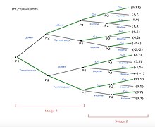
Steps for solving this Multi-Stage Game, with the extensive form as seen to the right:
- Backward induction starts to solve the game from the final nodes.
- Player 2 will observe 8 subgames from the final nodes to choose to “Go to Movie” or “Stay Home”
- Player 2 will make 4 comparisons in total. He will choose an option with the higher payoff.
- For example, considering the first subgame, payoff of 11 is higher than 7. Therefore, Player 2 chooses to “Go to Movie”.
- The method continues for every subgame.
- Once Player 2 completes his choices, Player 1 will make his choice based on selected subgames.
- The process is similar to Step 2. Player 1 compares her payoffs in order to make her choices.
- Subgames not selected by Player 2 from the previous step are no longer considered by both players because they are not optimal.
- For example, the choice to “Go to Movie” offers payoff of 9 (9,11) and choice to “Stay Home” offers payoff of 1 (1, 9). Player 1 will choose to “Go to Movie”.
- The process repeats for each player until the initial node is reached.
- For example, Player 2 will choose “Joker” because payoff of 11 (9, 11) is greater than “Terminator” with payoff of 6 (6, 6).
- For example, Player 1, at initial node, will select “Terminator” because it offers higher payoff of 11. Terminator: (11, 9) > Joker: (9, 11)
- To identify Subgame perfect equilibrium, we need to identify a route that selects optimal subgame at each information set.
- In this example, Player 1 chooses “Terminator” and Player 2 also chooses “Terminator”. Then, they both chooses to “Go to Movie”.
- The subgame perfect equilibrium leads to payoff of (11,9)
Backward induction in game theory: the ultimatum game[]
Backward induction is ‘the process of analyzing a game from the end to the beginning. As with solving for other Nash Equilibria, rationality of players and complete knowledge is assumed. The concept of backwards induction corresponds to this assumption that it is common knowledge that each player will act rationally with each decision node when she chooses an option — even if her rationality would imply that such a node will not be reached.’[10] Under the mutual assumption of rationality, therefore, backward induction allows each player to predict exactly what their opponent will do at every stage of the game.
In order to solve for a Subgame Perfect Equilibrium with backwards induction, the game should be written out in extensive form and then divided into subgames. Starting with the subgame furthest from the initial node, or starting point, the expected payoffs listed for this subgame are weighed and the rational player will select the option with the higher payoff for themselves. The highest payoff vector is selected and marked. Solve for the subgame perfect equilibrium by continually working backwards from subgame to subgame until arriving at the starting point. As this process progresses, your initial extensive form game will become shorter and shorter. The marked path of vectors is the subgame perfect equilibrium.[11]
Backward Induction Applied to the Ultimatum Game
Think of a game between two players where player 1 proposes to split a dollar with player 2. This is a famous, asymmetric game that is played sequentially called the ultimatum game. player one acts first by splitting the dollar however they see fit. Now, player two can either accept the portion they have been dealt by player one or reject the split. If player 2 accepts the split, then both player 1 and player 2 get the payoff according to that split. If player two decides to reject player 1’s offer, then both players get nothing. In other words, player 2 has veto power over player 1’s proposed allocation but applying the veto eliminates any reward for both players.[12] The strategy profile for this game therefore can be written as pairs (x, f(x)) for all x between 0 and 1, where f(x)) is a bi-valued function expressing whether x is accepted or not.
Consider the choice and response of player 2 given any arbitrary proposal by player 1, assuming that the offer is larger than $0. Using backward induction, surely we would expect player 2 to accept any payoff that is greater than or equal to $0. Accordingly, player 1 ought to propose giving player 2 as little as possible in order to gain the largest portion of the split. player 1 giving player 2 the smallest unit of money and keeping the rest for him/herself is the unique sub game perfect equilibrium. The ultimatum game does have several other Nash Equilibria which are not subgame perfect and therefore do not require backward induction.
The ultimatum game is an illustration of the usefulness of backward induction when considering infinite games; however, the game’s theoretically predicted results of the game are criticized. Empirical, experimental evidence has shown that the proposer very rarely offers $0 and player 2 sometimes even rejects offers greater than $0, presumably on grounds of fairness. What is deemed fair by player 2 varies by context and the pressure or presence of other players can mean that the game theoretic model can not necessarily predict what real people will choose.
In practice, subgame perfect equilibrium is not always achieved. According to Camerer, an American behavioral economist, player 2 “rejects offers of less than 20 percent of X about half the time, even though they end up with nothing.”[13] While backward induction would predict that the responder accepts any offer equal to or greater than zero, responders in reality are not rational players and therefore seem to care more about offer ‘fairness’ rather than potential monetary gains.
See also centipede game.
Backward induction in economics: the entry-decision problem[]
Consider a dynamic game in which the players are an incumbent firm in an industry and a potential entrant to that industry. As it stands, the incumbent has a monopoly over the industry and does not want to lose some of its market share to the entrant. If the entrant chooses not to enter, the payoff to the incumbent is high (it maintains its monopoly) and the entrant neither loses nor gains (its payoff is zero). If the entrant enters, the incumbent can "fight" or "accommodate" the entrant. It will fight by lowering its price, running the entrant out of business (and incurring exit costs — a negative payoff) and damaging its own profits. If it accommodates the entrant it will lose some of its sales, but a high price will be maintained and it will receive greater profits than by lowering its price (but lower than monopoly profits).
Consider if the best response of the incumbent is to accommodate if the entrant enters. If the incumbent accommodates, the best response of the entrant is to enter (and gain profit). Hence the strategy profile in which the entrant enters and the incumbent accommodates if the entrant enters is a Nash equilibrium consistent with backward induction. However, if the incumbent is going to fight, the best response of the entrant is to not enter, and if the entrant does not enter, it does not matter what the incumbent chooses to do in the hypothetical case that the entrant does enter. Hence the strategy profile in which the incumbent fights if the entrant enters, but the entrant does not enter is also a Nash equilibrium. However, were the entrant to deviate and enter, the incumbent's best response is to accommodate—the threat of fighting is not credible. This second Nash equilibrium can therefore be eliminated by backward induction.
Finding a Nash equilibrium in each decision-making process (subgame) constitutes as perfect subgame equilibria. Thus, these strategy profiles that depict subgame perfect equilibria exclude the possibility of actions like incredible threats that are used to "scare off" an entrant. If the incumbent threatens to start a Price war with an entrant, they are threatening to lower their prices from a monopoly price to slightly lower than the entrant's, which would be impractical, and incredible, if the entrant knew a price war would not actually happen since it would result in losses for both parties. Unlike a single agent optimization which includes equilibria that aren't feasible or optimal, a subgame perfect equilibrium accounts for the actions of another player, thus ensuring that no player reaches a subgame mistakenly. In this case, backwards induction yielding perfect subgame equilibria ensures that the entrant will not be convinced of the incumbent's threat knowing that it was not a best response in the strategy profile.[14]
Backward induction paradox: the unexpected hanging[]
The unexpected hanging paradox is a paradox related to backward induction. Suppose a prisoner is told that she will be hanged sometime between Monday and Friday of next week. However, the exact day will be a surprise (i.e. she will not know the night before that she will be executed the next day). The prisoner, interested in outsmarting her executioner, attempts to determine which day the execution will occur.
She reasons that it cannot occur on Friday, since if it had not occurred by the end of Thursday, she would know the execution would be on Friday. Therefore, she can eliminate Friday as a possibility. With Friday eliminated, she decides that it cannot occur on Thursday, since if it had not occurred on Wednesday, she would know that it had to be on Thursday. Therefore, she can eliminate Thursday. This reasoning proceeds until she has eliminated all possibilities. She concludes that she will not be hanged next week.
To her surprise, she is hanged on Wednesday. She made the mistake of assuming that she knew definitively whether the unknown future factor that would cause her execution was one that she could reason about.
Here the prisoner reasons by backward induction, but seems to come to a false conclusion. Note, however, that the description of the problem assumes it is possible to surprise someone who is performing backward induction. The mathematical theory of backward induction does not make this assumption, so the paradox does not call into question the results of this theory. Nonetheless, this paradox has received some substantial discussion by philosophers.
Backward induction and common knowledge of rationality[]
Backward induction works only if both players are rational, i.e., always select an action that maximizes their payoff. However, rationality is not enough: each player should also believe that all other players are rational. Even this is not enough: each player should believe that all other players know that all other players are rational. And so on ad infinitum. In other words, rationality should be common knowledge.[15]
Limited Backward Induction[]
Limited backward induction is a deviation from fully rational backward induction. It involves enacting the regular process of backward induction without perfect foresight. Theoretically, this occurs when one or more players have limited foresight and cannot perform backward induction through all terminal nodes.[16] Limited backward induction plays a much larger role in longer games as the effects of limited backward induction are more potent in later periods of games.

Experiments have shown that in sequential bargaining games, such as the Centipede game, subjects deviate from theoretical predictions and instead engage in limited backward induction. This deviation occurs as a result of bounded rationality, where players can only perfectly see a few stages ahead.[17] This allows for unpredictability in decisions and inefficiency in finding and achieving subgame perfect nash equilibria.
There are three broad hypotheses for this phenomenon;
- The presence of social factors (e.g. fairness)
- The presence of non-social factors (e.g. limited backward induction)
- Cultural difference
Violations of backward induction is predominantly attributed to the presence of social factors. However data-driven model predictions for sequential bargaining games (utilising the cognitive hierarchy model) have highlighted that in some games the presence of limited backward induction can play a dominant role.[18]
Within repeated public goods games, team behaviour is impacted by limited backward induction; where it is evident that team members' initial contributions are higher than contributions towards the end. Limited backward induction also influences how regularly free-riding occurs within a teams' public goods game. Early on when the effects of limited backward induction are low free-riding is less frequent, whilst towards the end, when effects are high, free riding becomes more frequent.[19]
Limited backward induction has also been tested for within a variant of the race game. In the game, players would sequentially choose integers inside a range and sum their choices until a target number is reached. Hitting the target earns that player a prize; the other loses. Partway through a series of games, a small prize was introduced. The majority of players then performed limited backward induction, as they solved for the small prize rather than for the original prize. Only a small fraction of players considered both prizes at the start.[20]
Notes[]
- ^ Rust, John (9 September 2016). Dynamic Programming. The New Palgrave Dictionary of Economics: Palgrave Macmillan. ISBN 978-1-349-95121-5.
- ^ Jerome Adda and Russell Cooper, "Dynamic Economics: Quantitative Methods and Applications", Section 3.2.1, page 28. MIT Press, 2003.
- ^ Mario Miranda and Paul Fackler, "Applied Computational Economics and Finance", Section 7.3.1, page 164. MIT Press, 2002.
- ^ Drew Fudenberg and Jean Tirole, "Game Theory", Section 3.5, page 92. MIT Press, 1991.
- ^ Mathematics of Chess, webpage by John MacQuarrie.
- ^ John von Neumann and Oskar Morgenstern, "Theory of Games and Economic Behavior", Section 15.3.1. Princeton University Press. Third edition, 1953. (First edition, 1944.)
- ^ Watson, Joel (2002). Strategy: an introduction to game theory (3 ed.). New York: W.W. Norton & Company. p. 63.
- ^ Watson, Joel (2002). Strategy: an introduction to game theory (3 ed.). New York: W.W. Norton & Company. pp. 186–187.
- ^ Watson, Joel (2002). Strategy: an introduction to game theory (3 ed.). New York: W.W. Norton & Company. p. 188.
- ^ http://web.mit.edu/14.12/www/02F_lecture7-9.pdf[bare URL PDF]
- ^ Rust, John (9 September 2016). Dynamic Programming. The New Palgrave Dictionary of Economics: Palgrave Macmillan. ISBN 978-1-349-95121-5.
- ^ Kamiński, Marek M. (2017). "Backward Induction: Merits And Flaws". Studies in Logic, Grammar and Rhetoric. 50 (1): 9–24. doi:10.1515/slgr-2017-0016.
- ^ Camerer, Colin F (1 November 1997). "Progress in Behavioral Game Theory". Journal of Economic Perspectives. 11 (4): 167–188. doi:10.1257/jep.11.4.167. JSTOR 2138470.
- ^ Rust J. (2008) Dynamic Programming. In: Palgrave Macmillan (eds) The New Palgrave Dictionary of Economics. Palgrave Macmillan, London
- ^ Aumann, Robert J. (January 1995). "Backward induction and common knowledge of rationality". Games and Economic Behavior. 8 (1): 6–19. doi:10.1016/S0899-8256(05)80015-6.
- ^ Marco Mantovani, 2015. "Limited backward induction: foresight and behavior in sequential games," Working Papers 289, University of Milano-Bicocca, Department of Economics
- ^ Ke, Shaowei (2019). "Boundedly rational backward induction". Theoretical Economics. 14 (1): 103–134. doi:10.3982/TE2402. S2CID 9053484.
- ^ Qu, Xia; Doshi, Prashant (1 March 2017). "On the role of fairness and limited backward induction in sequential bargaining games". Annals of Mathematics and Artificial Intelligence. 79 (1): 205–227. doi:10.1007/s10472-015-9481-7. S2CID 23565130.
- ^ Cox, Caleb A.; Stoddard, Brock (May 2018). "Strategic thinking in public goods games with teams". Journal of Public Economics. 161: 31–43. doi:10.1016/j.jpubeco.2018.03.007.
- ^ Mantovani, Marco (2013). "Limited backward induction". CiteSeerX 10.1.1.399.8991.
{{cite journal}}: Cite journal requires|journal=(help)
- Dynamic programming
- Game theory
- Inductive reasoning