Gamma distribution

Gamma

Probability density function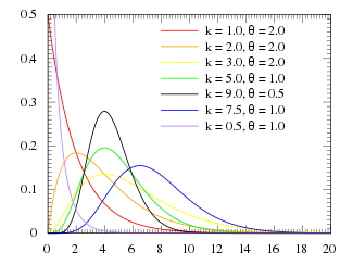
Cumulative distribution function
Parameters	k > 0 shape θ > 0 scale	α > 0 shape β > 0 rate
Support	${\displaystyle x\in (0,\infty )}$	${\displaystyle x\in (0,\infty )}$
PDF	${\displaystyle f(x)={\frac {1}{\Gamma (k)\theta ^{k}}}x^{k-1}e^{-{\frac {x}{\theta }}}}$	${\displaystyle f(x)={\frac {\beta ^{\alpha }}{\Gamma (\alpha )}}x^{\alpha -1}e^{-\beta x}}$
CDF	${\displaystyle F(x)={\frac {1}{\Gamma (k)}}\gamma \left(k,{\frac {x}{\theta }}\right)}$	${\displaystyle F(x)={\frac {1}{\Gamma (\alpha )}}\gamma (\alpha ,\beta x)}$
Mean	${\displaystyle k\theta }$	${\displaystyle {\frac {\alpha }{\beta }}}$
Median	No simple closed form	No simple closed form
Mode	${\displaystyle (k-1)\theta {\text{ for }}k\geq 1}$	${\displaystyle {\frac {\alpha -1}{\beta }}{\text{ for }}\alpha \geq 1}$
Variance	${\displaystyle k\theta ^{2}}$	${\displaystyle {\frac {\alpha }{\beta ^{2}}}}$
Skewness	${\displaystyle {\frac {2}{\sqrt {k}}}}$	${\displaystyle {\frac {2}{\sqrt {\alpha }}}}$
Ex. kurtosis	${\displaystyle {\frac {6}{k}}}$	${\displaystyle {\frac {6}{\alpha }}}$
Entropy	${\displaystyle {\begin{aligned}k&+\ln \theta +\ln \Gamma (k)\\&+(1-k)\psi (k)\end{aligned}}}$	${\displaystyle {\begin{aligned}\alpha &-\ln \beta +\ln \Gamma (\alpha )\\&+(1-\alpha )\psi (\alpha )\end{aligned}}}$
MGF	${\displaystyle (1-\theta t)^{-k}{\text{ for }}t<{\frac {1}{\theta }}}$	${\displaystyle \left(1-{\frac {t}{\beta }}\right)^{-\alpha }{\text{ for }}t<\beta }$
CF	${\displaystyle (1-\theta it)^{-k}}$	${\displaystyle \left(1-{\frac {it}{\beta }}\right)^{-\alpha }}$
Method of Moments	${\displaystyle k={\frac {E[X]^{2}}{V[X]}}\quad \quad }$ ${\displaystyle \theta ={\frac {V[X]}{E[X]}}\quad \quad }$	${\displaystyle \alpha ={\frac {E[X]^{2}}{V[X]}}}$ ${\displaystyle \beta ={\frac {E[X]}{V[X]}}}$

In probability theory and statistics, the gamma distribution is a two-parameter family of continuous probability distributions. The exponential distribution, Erlang distribution, and chi-square distribution are special cases of the gamma distribution. There are two different parameterizations in common use:

1. With a shape parameter k and a scale parameter θ.
2. With a shape parameter α = k and an inverse scale parameter β = 1/θ, called a rate parameter.

In each of these forms, both parameters are positive real numbers.

The gamma distribution is the maximum entropy probability distribution (both with respect to a uniform base measure and with respect to a 1/x base measure) for a random variable X for which E[X] = kθ = α/β is fixed and greater than zero, and E[ln(X)] = ψ(k) + ln(θ) = ψ(α) − ln(β) is fixed (ψ is the digamma function).^[1]

Definitions[]

The parameterization with k and θ appears to be more common in econometrics and certain other applied fields, where for example the gamma distribution is frequently used to model waiting times. For instance, in life testing, the waiting time until death is a random variable that is frequently modeled with a gamma distribution. See Hogg and Craig^[2] for an explicit motivation.

The parameterization with α and β is more common in Bayesian statistics, where the gamma distribution is used as a conjugate prior distribution for various types of inverse scale (rate) parameters, such as the λ of an exponential distribution or a Poisson distribution^[3] – or for that matter, the β of the gamma distribution itself. The closely related inverse-gamma distribution is used as a conjugate prior for scale parameters, such as the variance of a normal distribution.

If k is a positive integer, then the distribution represents an Erlang distribution; i.e., the sum of k independent exponentially distributed random variables, each of which has a mean of θ.

Characterization using shape α and rate β[]

The gamma distribution can be parameterized in terms of a shape parameter α = k and an inverse scale parameter β = 1/θ, called a rate parameter. A random variable X that is gamma-distributed with shape α and rate β is denoted

${\displaystyle X\sim \Gamma (\alpha ,\beta )\equiv \operatorname {Gamma} (\alpha ,\beta )}$

The corresponding probability density function in the shape-rate parametrization is

${\displaystyle {\begin{aligned}f(x;\alpha ,\beta )&={\frac {\beta ^{\alpha }x^{\alpha -1}e^{-\beta x}}{\Gamma (\alpha )}}\quad {\text{ for }}x>0\quad \alpha ,\beta >0,\\[6pt]\end{aligned}}}$

where ${\displaystyle \Gamma (\alpha )}$ is the gamma function. For all positive integers, ${\displaystyle \Gamma (\alpha )=(\alpha -1)!}$.

The cumulative distribution function is the regularized gamma function:

${\displaystyle F(x;\alpha ,\beta )=\int _{0}^{x}f(u;\alpha ,\beta )\,du={\frac {\gamma (\alpha ,\beta x)}{\Gamma (\alpha )}},}$

where ${\displaystyle \gamma (\alpha ,\beta x)}$ is the lower incomplete gamma function.

If α is a positive integer (i.e., the distribution is an Erlang distribution), the cumulative distribution function has the following series expansion:^[4]

${\displaystyle F(x;\alpha ,\beta )=1-\sum _{i=0}^{\alpha -1}{\frac {(\beta x)^{i}}{i!}}e^{-\beta x}=e^{-\beta x}\sum _{i=\alpha }^{\infty }{\frac {(\beta x)^{i}}{i!}}.}$

Characterization using shape k and scale θ[]

A random variable X that is gamma-distributed with shape k and scale θ is denoted by

${\displaystyle X\sim \Gamma (k,\theta )\equiv \operatorname {Gamma} (k,\theta )}$

Illustration of the gamma PDF for parameter values over k and x with θ set to 1, 2, 3, 4, 5 and 6. One can see each θ layer by itself here [2] as well as by k [3] and x. [4].

The probability density function using the shape-scale parametrization is

${\displaystyle f(x;k,\theta )={\frac {x^{k-1}e^{-{\frac {x}{\theta }}}}{\theta ^{k}\Gamma (k)}}\quad {\text{ for }}x>0{\text{ and }}k,\theta >0.}$

Here Γ(k) is the gamma function evaluated at k.

The cumulative distribution function is the regularized gamma function:

${\displaystyle F(x;k,\theta )=\int _{0}^{x}f(u;k,\theta )\,du={\frac {\gamma \left(k,{\frac {x}{\theta }}\right)}{\Gamma (k)}},}$

where ${\displaystyle \gamma \left(k,{\frac {x}{\theta }}\right)}$ is the lower incomplete gamma function.

It can also be expressed as follows, if k is a positive integer (i.e., the distribution is an Erlang distribution):^[4]

${\displaystyle F(x;k,\theta )=1-\sum _{i=0}^{k-1}{\frac {1}{i!}}\left({\frac {x}{\theta }}\right)^{i}e^{-x/\theta }=e^{-x/\theta }\sum _{i=k}^{\infty }{\frac {1}{i!}}\left({\frac {x}{\theta }}\right)^{i}.}$

Both parametrizations are common because either can be more convenient depending on the situation.

Properties[]

Skewness[]

The skewness of the gamma distribution only depends on its shape parameter, k, and it is equal to ${\displaystyle 2/{\sqrt {k}}.}$

Higher Moments[]

The nth raw moment is given by:

${\displaystyle \mathrm {E} [X^{n}]=\theta ^{n}{\frac {\Gamma (n+k)}{\Gamma (k)}}.}$

Median approximations and bounds[]

Bounds and asymptotic approximations to the median of the gamma distribution. The cyan colored region indicates the large gap between published lower and upper bounds.

Unlike the mode and the mean, which have readily calculable formulas based on the parameters, the median does not have a closed-form equation. The median for this distribution is defined as the value ${\displaystyle \nu }$ such that

${\displaystyle {\frac {1}{\Gamma (k)\theta ^{k}}}\int _{0}^{\nu }x^{k-1}e^{-x/\theta }dx={\frac {1}{2}}.}$

A rigorous treatment of the problem of determining an asymptotic expansion and bounds for the median of the gamma distribution was handled first by Chen and Rubin, who proved that (for ${\displaystyle \theta =1}$)

${\displaystyle k-{\frac {1}{3}}<\nu (k)<k,}$

where ${\displaystyle \mu (k)=k}$ is the mean and ${\displaystyle \nu (k)}$ is the median of the ${\displaystyle {\text{Gamma}}(k,1)}$ distribution.^[5] For other values of the scale parameter, the mean scales to ${\displaystyle \mu =k\theta }$, and the median bounds and approximations would be similarly scaled by ${\displaystyle \theta }$.

K. P. Choi found the first five terms in a Laurent series asymptotic approximation of the median by comparing the median to Ramanujan's ${\displaystyle \theta }$ function.^[6] Berg and Pedersen found more terms:^[7]

${\displaystyle \nu (k)=k-{\frac {1}{3}}+{\frac {8}{405k}}+{\frac {184}{25515k^{2}}}+{\frac {2248}{3444525k^{3}}}-{\frac {19006408}{15345358875k^{4}}}-O\left({\frac {1}{k^{5}}}\right)+\cdots }$

Two gamma distribution median asymptotes which are conjectured to be bounds (upper solid red and lower dashed red), of the from ${\displaystyle \nu (k)\approx 2^{-1/k}(A+k)}$, and an interpolation between them that makes an approximation (dotted red) that is exact at k = 1 and has maximum relative error of about 0.6%. The cyan shaded region is the remaining gap between upper and lower bounds (or conjectured bounds) including these new (as of 2021) conjectured bounds and the proven bounds in the previous figure.

Log–log plot of upper (solid) and lower (dashed) bounds to the median of a gamma distribution, and the gaps between them. The green, yellow, and cyan regions represent the gap before the Lyon 2021 paper. The green and yellow narrow that gap with the lower bounds that Lyon proved. The yellow is further narrowed by Lyon's conjectured bounds. Mostly within the yellow, closed-form rational-function-interpolated bounds are plotted, along with the numerically calculated value of the median (dotted). Tighter interpolated bounds exist but are not plotted, as they would not be resolved at this scale.

Partial sums of these series are good approximations for high enough ${\displaystyle k}$; they are not plotted in the figure, which is focused on the low-${\displaystyle k}$ region that is less well approximated.

Berg and Pedersen also proved many properties of the median, showed that it is a convex function of ${\displaystyle k}$,^[8] and that the asymptotic behavior near ${\displaystyle k=0}$ is ${\displaystyle \nu (k)\approx e^{-\gamma }2^{-1/k}}$ (where ${\displaystyle \gamma }$ is the Euler–Mascheroni constant), and that for all ${\displaystyle k>0}$ the median is bounded by ${\displaystyle k2^{-1/k}<\nu (k)<ke^{-1/3k}}$.^[7]

A closer linear upper bound, for ${\displaystyle k\geq 1}$ only, was provided in 2021 by Gaunt and Merkle,^[9] relying on the Berg and Pedersen result that the slope of ${\displaystyle \nu (k)}$ is everywhere less than 1:

${\displaystyle \nu (k)\leq k-1+\log 2~~}$ for ${\displaystyle k\geq 1}$ (with equality at ${\displaystyle k=1}$)

which can be extended to a bound for all ${\displaystyle k>0}$ by taking the max with the chord shown in the figure, since the median was proved convex.^[8]

An approximation to the median that is asymptotically accurate at high ${\displaystyle k}$ and reasonable down to ${\displaystyle k=0.5}$ or a bit lower follows from the Wilson–Hilferty transformation:

${\displaystyle \nu (k)=k\left(1-{\frac {1}{9k}}\right)^{3}}$

which goes negative for ${\displaystyle k<1/9}$.

In 2021, Lyon proposed several closed-form approximations of the form ${\displaystyle \nu (k)\approx 2^{-1/k}(A+Bk)}$. He conjectured closed-form values of ${\displaystyle A}$ and ${\displaystyle B}$ for which this approximation is an asymptotically tight upper or lower bound for all ${\displaystyle k>0}$. In particular:^[10]

${\displaystyle \nu _{L\infty }(k)=2^{-1/k}(\log 2-{\frac {1}{3}}+k)\quad }$ is a lower bound, asymptotically tight as ${\displaystyle k\to \infty }$

${\displaystyle \nu _{U}(k)=2^{-1/k}(e^{-\gamma }+k)\quad }$ is an upper bound, asymptotically tight as ${\displaystyle k\to 0}$

Lyon also derived two other lower bounds that are not closed-form expressions, including this one based on solving the integral expression substituting 1 for ${\displaystyle e^{-x}}$:

${\displaystyle \nu (k)>\left({\frac {2}{\Gamma (k+1)}}\right)^{-1/k}\quad }$ (approaching equality as ${\displaystyle k\to 0}$)

and the tangent line at ${\displaystyle k=1}$ where the derivative was found to be ${\displaystyle \nu ^{\prime }(1)\approx 0.9680448}$:

${\displaystyle \nu (k)\geq \nu (1)+(k-1)\nu ^{\prime }(1)\quad }$ (with equality at ${\displaystyle k=1}$)

${\displaystyle \nu (k)\geq \log(2)+(k-1)(\gamma -2{\textrm {Ei}}(-\log 2)-\log \log 2)}$

where Ei is the exponential integral.^[10]

Additionally, he showed that interpolations between bounds can provide excellent approximations or tighter bounds to the median, including an approximation that is exact at ${\displaystyle k=1}$ (where ${\displaystyle \nu (1)=\log 2}$) and has a maximum relative error less than 0.6%. Interpolated approximations and bounds are all of the form

${\displaystyle \nu (k)\approx {\tilde {g}}(k)\nu _{L\infty }(k)+(1-{\tilde {g}}(k))\nu _{U}(k)}$

where ${\displaystyle \nu (k)\approx {\tilde {g}}}$ is an interpolating function running monotonically from 0 at low ${\displaystyle k}$ to 1 at high ${\displaystyle k}$, approximating an ideal, or exact, interpolator ${\displaystyle g(k)}$:

${\displaystyle g(k)={\frac {\nu _{U}(k)-\nu (k)}{\nu _{U}(k)-\nu _{L\infty }(k)}}}$

For the simplest interpolating function considered, a first-order rational function

${\displaystyle {\tilde {g}}_{1}(k)={\frac {k}{b_{0}+k}}}$

the tightest lower bound has

${\displaystyle b_{0}={\frac {{\frac {8}{405}}+e^{-\gamma }\log 2-{\frac {\log ^{2}2}{2}}}{e^{-\gamma }-\log 2+{\frac {1}{3}}}}-\log 2\approx 0.143472}$

and the tightest upper bound has

${\displaystyle b_{0}={\frac {e^{-\gamma }-\log 2+{\frac {1}{3}}}{1-{\frac {e^{-\gamma }\pi ^{2}}{12}}}}\approx 0.374654}$

The interpolated bounds are plotted (mostly inside the yellow region) in the log–log plot shown. Even tighter bounds are available using different interpolating functions, but not usually with closed-form parameters like these.^[10]

Summation[]

If X_i has a Gamma(k_i, θ) distribution for i = 1, 2, ..., N (i.e., all distributions have the same scale parameter θ), then

${\displaystyle \sum _{i=1}^{N}X_{i}\sim \mathrm {Gamma} \left(\sum _{i=1}^{N}k_{i},\theta \right)}$

provided all X_i are independent.

For the cases where the X_i are independent but have different scale parameters see Mathai ^[11] or Moschopoulos.^[12]

The gamma distribution exhibits infinite divisibility.

Scaling[]

If

${\displaystyle X\sim \mathrm {Gamma} (k,\theta ),}$

then, for any c > 0,

${\displaystyle cX\sim \mathrm {Gamma} (k,c\,\theta ),}$ by moment generating functions,

or equivalently, if

${\displaystyle X\sim \mathrm {Gamma} \left(\alpha ,\beta \right)}$ (shape-rate parameterization)

${\displaystyle cX\sim \mathrm {Gamma} \left(\alpha ,{\frac {\beta }{c}}\right),}$

Indeed, we know that if X is an exponential r.v. with rate λ then cX is an exponential r.v. with rate λ/c; the same thing is valid with Gamma variates (and this can be checked using the moment-generating function, see, e.g.,these notes, 10.4-(ii)): multiplication by a positive constant c divides the rate (or, equivalently, multiplies the scale).

Exponential family[]

The gamma distribution is a two-parameter exponential family with natural parameters k − 1 and −1/θ (equivalently, α − 1 and −β), and natural statistics X and ln(X).

If the shape parameter k is held fixed, the resulting one-parameter family of distributions is a natural exponential family.

Logarithmic expectation and variance[]

One can show that

${\displaystyle \operatorname {E} [\ln(X)]=\psi (\alpha )-\ln(\beta )}$

or equivalently,

${\displaystyle \operatorname {E} [\ln(X)]=\psi (k)+\ln(\theta )}$

where ${\displaystyle \psi }$ is the digamma function. Likewise,

${\displaystyle \operatorname {var} [\ln(X)]=\psi ^{(1)}(\alpha )=\psi ^{(1)}(k)}$

where ${\displaystyle \psi ^{(1)}}$ is the trigamma function.

This can be derived using the exponential family formula for the moment generating function of the sufficient statistic, because one of the sufficient statistics of the gamma distribution is ln(x).

Information entropy[]

The information entropy is

${\displaystyle {\begin{aligned}\operatorname {H} (X)&=\operatorname {E} [-\ln(p(X))]\\&=\operatorname {E} [-\alpha \ln(\beta )+\ln(\Gamma (\alpha ))-(\alpha -1)\ln(X)+\beta X]\\&=\alpha -\ln(\beta )+\ln(\Gamma (\alpha ))+(1-\alpha )\psi (\alpha ).\end{aligned}}}$

In the k, θ parameterization, the information entropy is given by

${\displaystyle \operatorname {H} (X)=k+\ln(\theta )+\ln(\Gamma (k))+(1-k)\psi (k).}$

Kullback–Leibler divergence[]

Illustration of the Kullback–Leibler (KL) divergence for two gamma PDFs. Here β = β₀ + 1 which are set to 1, 2, 3, 4, 5 and 6. The typical asymmetry for the KL divergence is clearly visible.

The Kullback–Leibler divergence (KL-divergence), of Gamma(α_p, β_p) ("true" distribution) from Gamma(α_q, β_q) ("approximating" distribution) is given by^[13]

${\displaystyle {\begin{aligned}D_{\mathrm {KL} }(\alpha _{p},\beta _{p};\alpha _{q},\beta _{q})={}&(\alpha _{p}-\alpha _{q})\psi (\alpha _{p})-\log \Gamma (\alpha _{p})+\log \Gamma (\alpha _{q})\\&{}+\alpha _{q}(\log \beta _{p}-\log \beta _{q})+\alpha _{p}{\frac {\beta _{q}-\beta _{p}}{\beta _{p}}}.\end{aligned}}}$

Written using the k, θ parameterization, the KL-divergence of Gamma(k_p, θ_p) from Gamma(k_q, θ_q) is given by

${\displaystyle {\begin{aligned}D_{\mathrm {KL} }(k_{p},\theta _{p};k_{q},\theta _{q})={}&(k_{p}-k_{q})\psi (k_{p})-\log \Gamma (k_{p})+\log \Gamma (k_{q})\\&{}+k_{q}(\log \theta _{q}-\log \theta _{p})+k_{p}{\frac {\theta _{p}-\theta _{q}}{\theta _{q}}}.\end{aligned}}}$

Laplace transform[]

The Laplace transform of the gamma PDF is

${\displaystyle F(s)=(1+\theta s)^{-k}={\frac {\beta ^{\alpha }}{(s+\beta )^{\alpha }}}.}$

Related distributions[]

General[]

• Let ${\displaystyle X_{1},X_{2}\ldots X_{n}}$ be ${\displaystyle n}$ independent and identically distributed random variables following an exponential distribution with rate parameter λ, then ${\displaystyle \sum _{i}X_{i}}$ ~ Gamma(n, λ) where n is the shape parameter and λ is the rate, and ${\displaystyle {\bar {X}}={\frac {1}{n}}\sum _{i}X_{i}}$ ~ Gamma(n, n λ) where the rate changes n λ.
• If X ~ Gamma(1, 1/λ) (in the shape–scale parametrization), then X has an exponential distribution with rate parameter λ.
• If X ~ Gamma(ν/2, 2) (in the shape–scale parametrization), then X is identical to χ²(ν), the chi-squared distribution with ν degrees of freedom. Conversely, if Q ~ χ²(ν) and c is a positive constant, then cQ ~ Gamma(ν/2, 2c).
• If k is an integer, the gamma distribution is an Erlang distribution and is the probability distribution of the waiting time until the kth "arrival" in a one-dimensional Poisson process with intensity 1/θ. If

${\displaystyle X\sim \Gamma (k\in \mathbf {Z} ,\theta ),\qquad Y\sim \mathrm {Pois} \left({\frac {x}{\theta }}\right),}$

then

${\displaystyle P(X>x)=P(Y<k).}$

• If X has a Maxwell–Boltzmann distribution with parameter a, then

${\displaystyle X^{2}\sim \Gamma \left({\frac {3}{2}},2a^{2}\right)}$.

• If X ~ Gamma(k, θ), then ${\displaystyle \log {X}}$ follows an exponential-gamma (abbreviated exp-gamma) distribution.^[14] It is sometimes referred to as the log-gamma distribution.^[15] Formulas for its mean and variance are in the section #Logarithmic expectation and variance.
• If X ~ Gamma(k, θ), then ${\displaystyle {\sqrt {X}}}$ follows a generalized gamma distribution with parameters p = 2, d = 2k, and ${\displaystyle a={\sqrt {\theta }}}$^{[citation needed]}.
• More generally, if X ~ Gamma(k,θ), then ${\displaystyle X^{q}}$ for ${\displaystyle q>0}$ follows a generalized gamma distribution with parameters p = 1/q, d = k/q, and ${\displaystyle a=\theta ^{q}}$.
• If X ~ Gamma(k, θ) with shape k and scale θ, then 1/X ~ Inv-Gamma(k, θ⁻¹) (see Inverse-gamma distribution for derivation).
• Parametrization 1: If ${\displaystyle X_{k}\sim \Gamma (\alpha _{k},\theta _{k})\,}$ are independent, then ${\displaystyle {\frac {\alpha _{2}\theta _{2}X_{1}}{\alpha _{1}\theta _{1}X_{2}}}\sim \mathrm {F} (2\alpha _{1},2\alpha _{2})}$, or equivalently, ${\displaystyle {\frac {X_{1}}{X_{2}}}\sim \beta '\left(\alpha _{1},\alpha _{2},1,{\frac {\theta _{1}}{\theta _{2}}}\right)}$
• Parametrization 2: If ${\displaystyle X_{k}\sim \Gamma (\alpha _{k},\beta _{k})\,}$ are independent, then ${\displaystyle {\frac {\alpha _{2}\beta _{1}X_{1}}{\alpha _{1}\beta _{2}X_{2}}}\sim \mathrm {F} (2\alpha _{1},2\alpha _{2})}$, or equivalently, ${\displaystyle {\frac {X_{1}}{X_{2}}}\sim \beta '\left(\alpha _{1},\alpha _{2},1,{\frac {\beta _{2}}{\beta _{1}}}\right)}$
• If X ~ Gamma(α, θ) and Y ~ Gamma(β, θ) are independently distributed, then X/(X + Y) has a beta distribution with parameters α and β, and X/(X + Y) is independent of X + Y, which is Gamma(α + β, θ)-distributed.
• If X_i ~ Gamma(α_i, 1) are independently distributed, then the vector (X₁/S, ..., X_n/S), where S = X₁ + ... + X_n, follows a Dirichlet distribution with parameters α₁, ..., α_n.
• For large k the gamma distribution converges to normal distribution with mean μ = kθ and variance σ² = kθ².
• The gamma distribution is the conjugate prior for the precision of the normal distribution with known mean.
• The Wishart distribution is a multivariate generalization of the gamma distribution (samples are positive-definite matrices rather than positive real numbers).
• The gamma distribution is a special case of the generalized gamma distribution, the generalized integer gamma distribution, and the generalized inverse Gaussian distribution.
• Among the discrete distributions, the negative binomial distribution is sometimes considered the discrete analogue of the gamma distribution.
• Tweedie distributions – the gamma distribution is a member of the family of Tweedie exponential dispersion models.

Compound gamma[]

If the shape parameter of the gamma distribution is known, but the inverse-scale parameter is unknown, then a gamma distribution for the inverse scale forms a conjugate prior. The compound distribution, which results from integrating out the inverse scale, has a closed-form solution, known as the compound gamma distribution.^[16]

If instead the shape parameter is known but the mean is unknown, with the prior of the mean being given by another gamma distribution, then it results in K-distribution.

Statistical inference[]

Parameter estimation[]

Maximum likelihood estimation[]

The likelihood function for N iid observations (x₁, ..., x_N) is

${\displaystyle L(k,\theta )=\prod _{i=1}^{N}f(x_{i};k,\theta )}$

from which we calculate the log-likelihood function

${\displaystyle \ell (k,\theta )=(k-1)\sum _{i=1}^{N}\ln(x_{i})-\sum _{i=1}^{N}{\frac {x_{i}}{\theta }}-Nk\ln(\theta )-N\ln(\Gamma (k))}$

Finding the maximum with respect to θ by taking the derivative and setting it equal to zero yields the maximum likelihood estimator of the θ parameter:

${\displaystyle {\hat {\theta }}={\frac {1}{kN}}\sum _{i=1}^{N}x_{i}}$

Substituting this into the log-likelihood function gives

${\displaystyle \ell =(k-1)\sum _{i=1}^{N}\ln(x_{i})-Nk-Nk\ln \left({\frac {\sum x_{i}}{kN}}\right)-N\ln(\Gamma (k))}$

Finding the maximum with respect to k by taking the derivative and setting it equal to zero yields

${\displaystyle \ln(k)-\psi (k)=\ln \left({\frac {1}{N}}\sum _{i=1}^{N}x_{i}\right)-{\frac {1}{N}}\sum _{i=1}^{N}\ln(x_{i})}$

where ψ is the digamma function. There is no closed-form solution for k. The function is numerically very well behaved, so if a numerical solution is desired, it can be found using, for example, Newton's method. An initial value of k can be found either using the method of moments, or using the approximation

${\displaystyle \ln(k)-\psi (k)\approx {\frac {1}{2k}}\left(1+{\frac {1}{6k+1}}\right)}$

If we let

${\displaystyle s=\ln \left({\frac {1}{N}}\sum _{i=1}^{N}x_{i}\right)-{\frac {1}{N}}\sum _{i=1}^{N}\ln(x_{i})}$

then k is approximately

${\displaystyle k\approx {\frac {3-s+{\sqrt {(s-3)^{2}+24s}}}{12s}}}$

which is within 1.5% of the correct value.^[17] An explicit form for the Newton–Raphson update of this initial guess is:^[18]

${\displaystyle k\leftarrow k-{\frac {\ln(k)-\psi (k)-s}{{\frac {1}{k}}-\psi ^{\prime }(k)}}.}$

Closed-form estimators[]

Consistent closed-form estimators of k and θ exists that are derived from the likelihood of the generalized gamma distribution.^[19]

The estimate for the shape k is

${\displaystyle {\hat {k}}={\frac {N\sum _{i=1}^{N}x_{i}}{N\sum _{i=1}^{N}x_{i}\ln(x_{i})-\sum _{i=1}^{N}\ln(x_{i})\sum _{i=1}^{N}x_{i}}}}$

and the estimate for the scale θ is

${\displaystyle {\hat {\theta }}={\frac {1}{N^{2}}}\left(N\sum _{i=1}^{N}x_{i}\ln(x_{i})-\sum _{i=1}^{N}\ln(x_{i})\sum _{i=1}^{N}x_{i}\right)}$

If the rate parameterization is used, the estimate of ${\displaystyle {\hat {\beta }}={\frac {1}{\hat {\theta }}}}$.

These estimators are not strictly maximum likelihood estimators, but are instead referred to as mixed type log-moment estimators. They have however similar efficiency as the maximum likelihood estimators.

Although these estimators are consistent, they have a small bias. A bias-corrected variant of the estimator for the scale θ is

${\displaystyle {\tilde {\theta }}={\frac {N}{N-1}}{\hat {\theta }}}$

A bias correction for the shape parameter k is given as^[20]

${\displaystyle {\tilde {k}}={\hat {k}}-{\frac {1}{N}}\left(3{\hat {k}}-{\frac {2}{3}}\left({\frac {\hat {k}}{1+{\hat {k}}}}\right)-{\frac {4}{5}}{\frac {\hat {k}}{(1+{\hat {k}})^{2}}}\right)}$

Bayesian minimum mean squared error[]

With known k and unknown θ, the posterior density function for theta (using the standard scale-invariant prior for θ) is

${\displaystyle P(\theta \mid k,x_{1},\dots ,x_{N})\propto {\frac {1}{\theta }}\prod _{i=1}^{N}f(x_{i};k,\theta )}$

Denoting

${\displaystyle y\equiv \sum _{i=1}^{N}x_{i},\qquad P(\theta \mid k,x_{1},\dots ,x_{N})=C(x_{i})\theta ^{-Nk-1}e^{-y/\theta }}$

Integration with respect to θ can be carried out using a change of variables, revealing that 1/θ is gamma-distributed with parameters α = Nk, β = y.

${\displaystyle \int _{0}^{\infty }\theta ^{-Nk-1+m}e^{-y/\theta }\,d\theta =\int _{0}^{\infty }x^{Nk-1-m}e^{-xy}\,dx=y^{-(Nk-m)}\Gamma (Nk-m)\!}$

The moments can be computed by taking the ratio (m by m = 0)

${\displaystyle \operatorname {E} [x^{m}]={\frac {\Gamma (Nk-m)}{\Gamma (Nk)}}y^{m}}$

which shows that the mean ± standard deviation estimate of the posterior distribution for θ is

${\displaystyle {\frac {y}{Nk-1}}\pm {\sqrt {\frac {y^{2}}{(Nk-1)^{2}(Nk-2)}}}.}$

Bayesian inference[]

Conjugate prior[]

In Bayesian inference, the gamma distribution is the conjugate prior to many likelihood distributions: the Poisson, exponential, normal (with known mean), Pareto, gamma with known shape σ, inverse gamma with known shape parameter, and Gompertz with known scale parameter.

The gamma distribution's conjugate prior is:^[21]

${\displaystyle p(k,\theta \mid p,q,r,s)={\frac {1}{Z}}{\frac {p^{k-1}e^{-\theta ^{-1}q}}{\Gamma (k)^{r}\theta ^{ks}}},}$

where Z is the normalizing constant, which has no closed-form solution. The posterior distribution can be found by updating the parameters as follows:

${\displaystyle {\begin{aligned}p'&=p\prod \nolimits _{i}x_{i},\\q'&=q+\sum \nolimits _{i}x_{i},\\r'&=r+n,\\s'&=s+n,\end{aligned}}}$

where n is the number of observations, and x_i is the ith observation.

Occurrence and applications[]

The gamma distribution has been used to model the size of insurance claims^[22] and rainfalls.^[23] This means that aggregate insurance claims and the amount of rainfall accumulated in a reservoir are modelled by a gamma process – much like the exponential distribution generates a Poisson process.

The gamma distribution is also used to model errors in multi-level Poisson regression models, because a mixture of Poisson distributions with gamma distributed rates has a known closed form distribution, called negative binomial.

In wireless communication, the gamma distribution is used to model the multi-path fading of signal power;^{[citation needed]} see also Rayleigh distribution and Rician distribution.

In oncology, the age distribution of cancer incidence often follows the gamma distribution, whereas the shape and scale parameters predict, respectively, the number of driver events and the time interval between them.^[24][25]

In neuroscience, the gamma distribution is often used to describe the distribution of inter-spike intervals.^[26][27]

In bacterial gene expression, the copy number of a protein often follows the gamma distribution, where the scale and shape parameter are, respectively, the mean number of bursts per cell cycle and the mean number of protein molecules produced by a single mRNA during its lifetime.^[28]

In genomics, the gamma distribution was applied in peak calling step (i.e. in recognition of signal) in ChIP-chip^[29] and ChIP-seq^[30] data analysis.

The gamma distribution is widely used as a conjugate prior in Bayesian statistics. It is the conjugate prior for the precision (i.e. inverse of the variance) of a normal distribution. It is also the conjugate prior for the exponential distribution.

Generating gamma-distributed random variables[]

Given the scaling property above, it is enough to generate gamma variables with θ = 1 as we can later convert to any value of β with simple division.

Suppose we wish to generate random variables from Gamma(n + δ, 1), where n is a non-negative integer and 0 < δ < 1. Using the fact that a Gamma(1, 1) distribution is the same as an Exp(1) distribution, and noting the method of generating exponential variables, we conclude that if U is uniformly distributed on (0, 1], then −ln(U) is distributed Gamma(1, 1) (i.e. inverse transform sampling). Now, using the "α-addition" property of gamma distribution, we expand this result:

${\displaystyle -\sum _{k=1}^{n}\ln U_{k}\sim \Gamma (n,1)}$

where U_k are all uniformly distributed on (0, 1] and independent. All that is left now is to generate a variable distributed as Gamma(δ, 1) for 0 < δ < 1 and apply the "α-addition" property once more. This is the most difficult part.

Random generation of gamma variates is discussed in detail by Devroye,^{[31]: 401–428} noting that none are uniformly fast for all shape parameters. For small values of the shape parameter, the algorithms are often not valid.^[31]: 406 For arbitrary values of the shape parameter, one can apply the Ahrens and Dieter^[32] modified acceptance–rejection method Algorithm GD (shape k ≥ 1), or transformation method^[33] when 0 < k < 1. Also see Cheng and Feast Algorithm GKM 3^[34] or Marsaglia's squeeze method.^[35]

The following is a version of the Ahrens-Dieter acceptance–rejection method:^[32]

1. Generate U, V and W as iid uniform (0, 1] variates.
2. If ${\displaystyle U\leq {\frac {e}{e+\delta }}}$ then ${\displaystyle \xi =V^{1/\delta }}$ and ${\displaystyle \eta =W\xi ^{\delta -1}}$. Otherwise, ${\displaystyle \xi =1-\ln V}$ and ${\displaystyle \eta =We^{-\xi }}$.
3. If ${\displaystyle \eta >\xi ^{\delta -1}e^{-\xi }}$ then go to step 1.
4. ξ is distributed as Γ(δ, 1).

A summary of this is

${\displaystyle \theta \left(\xi -\sum _{i=1}^{\lfloor k\rfloor }\ln(U_{i})\right)\sim \Gamma (k,\theta )}$

where ${\displaystyle \scriptstyle \lfloor k\rfloor }$ is the integer part of k, ξ is generated via the algorithm above with δ = {k} (the fractional part of k) and the U_k are all independent.

While the above approach is technically correct, Devroye notes that it is linear in the value of k and in general is not a good choice. Instead he recommends using either rejection-based or table-based methods, depending on context.^{[31]: 401–428}

For example, Marsaglia's simple transformation-rejection method relying on one normal variate X and one uniform variate U:^[36]

1. Set ${\displaystyle d=a-{\frac {1}{3}}}$ and ${\displaystyle c={\frac {1}{\sqrt {9d}}}}$.
2. Set ${\displaystyle v=(1+cX)^{3}}$.
3. If ${\displaystyle v>0}$ and ${\displaystyle \ln U<{\frac {X^{2}}{2}}+d-dv+d\ln v}$ return ${\displaystyle dv}$, else go back to step 2.

With ${\displaystyle 1\leq a=\alpha =k}$ generates a gamma distributed random number in time that is approximately constant with k. The acceptance rate does depend on k, with an acceptance rate of 0.95, 0.98, and 0.99 for k=1, 2, and 4. For k < 1, one can use ${\displaystyle \gamma _{\alpha }=\gamma _{1+\alpha }U^{1/\alpha }}$ to boost k to be usable with this method.

Notes[]

External links[]

The Wikibook Statistics has a page on the topic of: Gamma distribution

• "Gamma-distribution", Encyclopedia of Mathematics, EMS Press, 2001 [1994]
• Weisstein, Eric W. "Gamma distribution". MathWorld.
• ModelAssist (2017) Uses of the gamma distribution in risk modeling, including applied examples in Excel.
• Engineering Statistics Handbook