Lineweaver–Burk plot

An example of a Lineweaver-Burk plot.

In biochemistry, the Lineweaver–Burk plot (or double reciprocal plot) is a graphical representation of the Lineweaver–Burk equation of enzyme kinetics, described by Hans Lineweaver and Dean Burk in 1934.^[1] The Lineweaver–Burk plot for inhibited enzymes can be compared to no inhibitor to determine how the inhibitor is competing with the enzyme.^[2]

The Lineweaver–Burk plot is correct when the enzyme kinetics obey ideal second- order kinetics, however non-linear regression is needed for systems that do not behave ideally. The double reciprocal plot distorts the error structure of the data, and is therefore not the most accurate tool for the determination of enzyme kinetic parameters.^[3] Non-linear regression or alternative linear forms of the Michaelis–Menten equation such as the Hanes-Woolf plot or Eadie–Hofstee plot are generally used for the calculation of parameters.^[4]

Definitions for Interpreting Plot[]

[S]: substrate concentration. The independent axis of Lineweaver- Burk plot is the reciprocal of substrate concentration.^[2]

V₀ or V: initial velocity of an enzyme inhibited reaction. The dependent axis of the Lineweaver- Burk plot is the reciprocal of velocity.^[5]

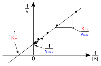
V_max: maximum velocity of the reaction. The y-intercept of the Lineweaver- Burk plot is the reciprocal of maximum velocity.^[2]

K_M: Michaelis-Menten constant or enzyme affinity. The lower the K_M the higher the affinity. Graphically the x-intercept of the line is -1/K_M.^[5]

K_cat: turnover number, or reactions per unit time. The lower the K_cat the slower the reaction. K_cat=V_max/[Enzyme]. Graphically this can be evaluated by looking at V_max.^[2]

Catalytic Efficiency= K_cat/K_M . A fast catalyst and high affinity results in best catalytic efficiency.^[5]

${\displaystyle {\ce {\alpha}}}$ = ${\displaystyle 1+[I]/K_{I}}$ where ${\displaystyle [I]}$ is the concentration of inhibition and ${\displaystyle K_{I}}$ is the inhibitor constant. Alpha determines the degree that binding of an inhibitor effects enzyme kinetics of a substrate, it always has a positive value.^[5]

Derivation[]

The plot provides a useful graphical method for analysis of the Michaelis–Menten equation, as it is difficult to determine precisely the V_max of an enzyme-catalysed reaction:

${\displaystyle V={\frac {V_{\max }[S]}{K_{m}+[S]}}}$

Taking the reciprocal gives:

${\displaystyle {1 \over V}={{K_{m}+[S]} \over V_{\max }[S]}={K_{m} \over V_{\max }}{1 \over [S]}+{1 \over V_{\max }}}$

The Lineweaver–Burk plot puts 1/[S] on the x-axis and 1/V on the y-axis.^[6]

Applications[]

_{Enzyme Inhibition displayed using Lineweaver-Burk (double reciprocal plots)}

When used for determining the type of enzyme inhibition, the Lineweaver–Burk plot can distinguish competitive, pure non-competitive and uncompetitive inhibitors. The various modes of inhibition can be compared to the uninhibited reaction.

Competitive Inhibition[]

V_max is unaffected by competitive inhibitors. Therefore competitive inhibitors have the same y-intercept as uninhibited enzymes (since V_max is unaffected by competitive inhibitors the inverse of V_max also doesn't change).

Competitive inhibition increases the K_M ,or lowers substrate affinity. The K_M inhibited is ${\displaystyle {\ce {\alpha}}}$ K_M.^[5] Graphically this can be seen as the inhibited enzyme having a larger x-intercept.^[2] The slopes of competitively inhibited enzymes and non-inhibited enzymes are different. Competitive inhibition is shown on the far left image.

Pure Noncompetitive Inhibition[]

With pure noncompetitive inhibition V_max is lowered with inhibition. V_max inhibited is ${\displaystyle {\ce {\alpha}}}$ V_max.^[5] This can be seen on the Lineweaver–Burk plot as an increased y-intercept with inhibition, as the reciprocal is plotted.^[7]

Pure noncompetitive inhibition does not effect substrate affinity, therefore K_M remains unchanged. Graphically this can be seen in that enzymes with pure noncompetitive inhibition intersect with non-inhibited enzymes at the x-axis.^[2] The slopes of pure noncompetitive inhibited enzymes and non-inhibited enzymes are different.^[7] Pure noncompetitive inhibition is shown in the image far right image.

Mixed Inhibition[]

Pure noncompetitive inhibition is rare, meaning mixed inhibition is more likely to result. In the case of mixed inhibition V_max and K_M are both effected at non-proportional rate. In most cases V_max is decreased, while K_M is increased, meaning affinity usually decreases with mixed inhibition. The lines of mixed inhibition and no inhibition intersect somewhere between the x- axis and y- axis, but never on an axis with mixed inhibition.^[5]  

Uncompetitive Inhibition[]

V_max decreases with uncompetitive inhibition. V_max inhibited is ${\displaystyle {\ce {\alpha}}}$ V_max.^[5] This can be seen on the Lineweaver–Burk plot as an increased y-intercept with inhibition, as the reciprocal is plotted.^[7] This relationship is seen in both uncompetitive inhibition and pure competitive inhibition.^[5]

Substrate affinity increases with uncompetitive inhibition, or lowers K_M. The inhibited K_M is K_M / ${\displaystyle {\ce {\alpha}}}$. Graphically this means that enzymes with uncompetitive inhibition will have a smaller x-intercept than non inhibited enzymes.^[5] Despite the x-intercept and y-intercept of uncompetitive inhibition both changing, the slope remains constant. Graphically uncompetitive inhibition can be identified in that the line of inhibited enzyme is parallel to non-inhibited enzyme. Uncompetitive inhibition is shown in the middle image.

Problems with Lineweaver-Burk[]

While the Lineweaver-Burk is useful for determining important variables in enzyme kinetics, it is prone to error. The y-axis of the plot takes the reciprocal of the rate of reaction, meaning small errors in measurement are more noticeable.^[8] Additionally because most points on the plot are found far to the right of the y-axis. large values of [S] (and hence small values for 1/[S] on the plot) are often not possible due to limited solubility.^[8]

See also[]

• Michaelis–Menten kinetics
• Eadie–Hofstee diagram
• Hanes–Woolf plot

References[]

External links[]

• NIH guide, enzyme assay development and analysis