Dragon curve
A dragon curve is any member of a family of self-similar fractal curves, which can be approximated by recursive methods such as Lindenmayer systems. The dragon curve is probably most commonly thought of as the shape that is generated from repeatedly folding a strip of paper in half, although there are other curves that are called dragon curves that are generated differently.
Heighway dragon[]
The Heighway dragon (also known as the Harter–Heighway dragon or the Jurassic Park dragon) was first investigated by NASA physicists John Heighway, Bruce Banks, and William Harter. It was described by Martin Gardner in his Scientific American column Mathematical Games in 1967. Many of its properties were first published by Chandler Davis and Donald Knuth. It appeared on the section title pages of the Michael Crichton novel Jurassic Park.[1]
Construction[]


The Heighway dragon can be constructed from a base line segment by repeatedly replacing each segment by two segments with a right angle and with a rotation of 45° alternatively to the right and to the left:[2]

The Heighway dragon is also the limit set of the following iterated function system in the complex plane:


with the initial set of points .

Using pairs of real numbers instead, this is the same as the two functions consisting of


[Un]folding the dragon[]
The Heighway dragon curve can be constructed by folding a strip of paper, which is how it was originally discovered.[1] Take a strip of paper and fold it in half to the right. Fold it in half again to the right. If the strip was opened out now, unbending each fold to become a 90-degree turn, the turn sequence would be RRL, i.e. the second iteration of the Heighway dragon. Fold the strip in half again to the right, and the turn sequence of the unfolded strip is now RRLRRLL – the third iteration of the Heighway dragon. Continuing folding the strip in half to the right to create further iterations of the Heighway dragon (in practice, the strip becomes too thick to fold sharply after four or five iterations).

The folding patterns of this sequence of paper strips, as sequences of right (R) and left (L) folds, are:
- 1st iteration: R
- 2nd iteration: R R L
- 3rd iteration: R R L R R L L
- 4th iteration: R R L R R L L R R R L L R L L.
Each iteration can be found by copying the previous iteration, then an R, then a second copy of the previous iteration in reverse order with the L and R letters swapped.[1]
Properties[]
- Many self-similarities can be seen in the Heighway dragon curve. The most obvious is the repetition of the same pattern tilted by 45° and with a reduction ratio of . Based on these self-similarities, many of its lengths are simple rational numbers.


- The dragon curve can tile the plane. One possible tiling replaces each edge of a square tiling with a dragon curve, using the recursive definition of the dragon starting from a line segment. The initial direction to expand each segment can be determined from a checkerboard coloring of a square tiling, expanding vertical segments into black tiles and out of white tiles, and expanding horizontal segments into white tiles and out of black ones.[3]
- As a non-self-crossing space-filling curve, the dragon curve has fractal dimension exactly 2. For a dragon curve with initial segment length 1, its area is 1/2, as can be seen from its tilings of the plane.[1]
- The boundary of the set covered by the dragon curve has infinite length, with fractal dimension whereis the real solution of the equation [4]


Twindragon[]

The twindragon (also known as the Davis–Knuth dragon) can be constructed by placing two Heighway dragon curves back to back. It is also the limit set of the following iterated function system:

where the initial shape is defined by the following set .

It can be also written as a Lindenmayer system – it only needs adding another section in initial string:
- angle 90°
- initial string FX+FX+
- string rewriting rules
- X ↦ X+YF
- Y ↦ FX−Y.
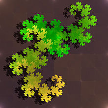
Terdragon[]

The terdragon can be written as a Lindenmayer system:
- angle 120°
- initial string F
- string rewriting rules
- F ↦ F+F−F.
It is the limit set of the following iterated function system:


Lévy dragon[]
The Lévy C curve is sometimes known as the Lévy dragon.[5]
 Lévy C curve. |
Variants[]
It is possible to change the turn angle from 90° to other angles. Changing to 120° yields a structure of triangles, while 60° gives the following curve:

A discrete dragon curve can be converted to a dragon polyomino as shown. Like discrete dragon curves, dragon polyominoes approach the fractal dragon curve as a limit.

Occurrences of the dragon curve in solution sets[]
Having obtained the set of solutions to a linear differential equation, any linear combination of the solutions will, because of the superposition principle, also obey the original equation. In other words, new solutions are obtained by applying a function to the set of existing solutions. This is similar to how an iterated function system produces new points in a set, though not all IFS are linear functions. In a conceptually similar vein, a set of Littlewood polynomials can be arrived at by such iterated applications of a set of functions.
A Littlewood polynomial is a polynomial: where all .


For some we define the following functions:


Starting at z=0 we can generate all Littlewood polynomials of degree d using these functions iteratively d+1 times.[6] For instance:

It can be seen that for , the above pair of functions is equivalent to the IFS formulation of the Heighway dragon. That is, the Heighway dragon, iterated to a certain iteration, describe the set of all Littlewood polynomials up to a certain degree, evaluated at the point . Indeed, when plotting a sufficiently high number of roots of the Littlewood polynomials, structures similar to the dragon curve appear at points close to these coordinates.[6][7][8]

See also[]
References[]
- ^ Jump up to: a b c d Tabachnikov, Sergei (2014), "Dragon curves revisited", The Mathematical Intelligencer, 36 (1): 13–17, doi:10.1007/s00283-013-9428-y, MR 3166985
- ^ Edgar, Gerald (2008), "Heighway's Dragon", Measure, Topology, and Fractal Geometry, Undergraduate Texts in Mathematics (2nd ed.), New York: Springer, pp. 20–22, doi:10.1007/978-0-387-74749-1, ISBN 978-0-387-74748-4, MR 2356043
- ^ Edgar (2008), "Heighway’s Dragon Tiles the Plane", pp. 74–75.
- ^ Edgar (2008), "Heighway Dragon Boundary", pp. 194–195.
- ^ Bailey, Scott; Kim, Theodore; Strichartz, Robert S. (2002), "Inside the Lévy dragon", The American Mathematical Monthly, 109 (8): 689–703, doi:10.2307/3072395, JSTOR 3072395, MR 1927621.
- ^ Jump up to: a b http://golem.ph.utexas.edu/category/2009/12/this_weeks_finds_in_mathematic_46.html
- ^ http://math.ucr.edu/home/baez/week285.html
- ^ http://johncarlosbaez.wordpress.com/2011/12/11/the-beauty-of-roots/
External links[]
| Wikimedia Commons has media related to Dragon curve. |


- Fractal curves
- Paper folding
- L-systems