Barnsley fern

Barnsley fern.

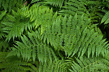
The Barnsley fern is a fractal named after the British mathematician Michael Barnsley who first described it in his book Fractals Everywhere.^[1] He made it to resemble the black spleenwort, Asplenium adiantum-nigrum.

History[]

The fern is one of the basic examples of self-similar sets, i.e. it is a mathematically generated pattern that can be reproducible at any magnification or reduction. Like the Sierpinski triangle, the Barnsley fern shows how graphically beautiful structures can be built from repetitive uses of mathematical formulas with computers. Barnsley's 1988 book Fractals Everywhere is based on the course which he taught for undergraduate and graduate students in the School of Mathematics, Georgia Institute of Technology, called Fractal Geometry. After publishing the book, a second course was developed, called Fractal Measure Theory.^[1] Barnsley's work has been a source of inspiration to graphic artists attempting to imitate nature with mathematical models.

Barnsley fern plotted with Processing

The fern code developed by Barnsley is an example of an iterated function system (IFS) to create a fractal. This follows from the collage theorem. He has used fractals to model a diverse range of phenomena in science and technology, but most specifically plant structures.

IFSs provide models for certain plants, leaves, and ferns, by virtue of the self-similarity which often occurs in branching structures in nature. But nature also exhibits randomness and variation from one level to the next; no two ferns are exactly alike, and the branching fronds become leaves at a smaller scale. V-variable fractals allow for such randomness and variability across scales, while at the same time admitting a continuous dependence on parameters which facilitates geometrical modelling. These factors allow us to make the hybrid biological models... ...we speculate that when a V -variable geometrical fractal model is found that has a good match to the geometry of a given plant, then there is a specific relationship between these code trees and the information stored in the genes of the plant.

—Michael Barnsley et al.^[2]

Construction[]

Real lady ferns.

Barnsley's fern uses four affine transformations. The formula for one transformation is the following:

f(x,y)={\begin{bmatrix}a&b\\c&d\end{bmatrix}}{\begin{bmatrix}x\\y\end{bmatrix}}+{\begin{bmatrix}e\\f\end{bmatrix}}

Barnsley shows the IFS code for his Black Spleenwort fern fractal as a matrix of values shown in a table.^[3] In the table, the columns "a" through "f" are the coefficients of the equation, and "p" represents the probability factor.

w	a	b	c	d	f	p	Portion generated
ƒ₁	0	0	0	0.16	0	0.01	Stem
ƒ₂	0.85	0.04	−0.04	0.85	1.60	0.85	Successively smaller leaflets
ƒ₃	0.20	−0.26	0.23	0.22	1.60	0.07	Largest left-hand leaflet
ƒ₄	−0.15	0.28	0.26	0.24	0.44	0.07	Largest right-hand leaflet

These correspond to the following transformations:

f_{1}(x,y)={\begin{bmatrix}\ 0.00&\ 0.00\ \\0.00&\ 0.16\end{bmatrix}}{\begin{bmatrix}\ x\\y\end{bmatrix}}

f_{2}(x,y)={\begin{bmatrix}\ 0.85&\ 0.04\ \\-0.04&\ 0.85\end{bmatrix}}{\begin{bmatrix}\ x\\y\end{bmatrix}}+{\begin{bmatrix}\ 0.00\\1.60\end{bmatrix}}

f_{3}(x,y)={\begin{bmatrix}\ 0.20&\ -0.26\ \\0.23&\ 0.22\end{bmatrix}}{\begin{bmatrix}\ x\\y\end{bmatrix}}+{\begin{bmatrix}\ 0.00\\1.60\end{bmatrix}}

f_{4}(x,y)={\begin{bmatrix}\ -0.15&\ 0.28\ \\0.26&\ 0.24\end{bmatrix}}{\begin{bmatrix}\ x\\y\end{bmatrix}}+{\begin{bmatrix}\ 0.00\\0.44\end{bmatrix}}

Computer generation[]

Fractal fern in four states of construction. Highlighted triangles show how the half of one leaflet is transformed to half of one whole leaf or frond.

Though Barnsley's fern could in theory be plotted by hand with a pen and graph paper, the number of iterations necessary runs into the tens of thousands, which makes use of a computer practically mandatory. Many different computer models of Barnsley's fern are popular with contemporary mathematicians. As long as math is programmed correctly using Barnsley's matrix of constants, the same fern shape will be produced.

The first point drawn is at the origin (x₀ = 0, y₀ = 0) and then the new points are iteratively computed by randomly applying one of the following four coordinate transformations:^[4]^[5]

ƒ₁

x_{n + 1} = 0

y_{n + 1} = 0.16 y_n.

This coordinate transformation is chosen 1% of the time and just maps any point to a point in the first line segment at the base of the stem. This part of the figure is the first to be completed during the course of iterations.

ƒ₂

x_{n + 1} = 0.85 x_n + 0.04 y_n

y_{n + 1} = −0.04 x_n + 0.85 y_n + 1.6.

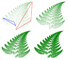
This coordinate transformation is chosen 85% of the time and maps any point inside the leaflet represented by the red triangle to a point inside the opposite, smaller leaflet represented by the blue triangle in the figure.

ƒ₃

x_{n + 1} = 0.2 x_n − 0.26 y_n

y_{n + 1} = 0.23 x_n + 0.22 y_n + 1.6.

This coordinate transformation is chosen 7% of the time and maps any point inside the leaflet (or pinna) represented by the blue triangle to a point inside the alternating corresponding triangle across the stem (it flips it).

ƒ₄

x_{n + 1} = −0.15 x_n + 0.28 y_n

y_{n + 1} = 0.26 x_n + 0.24 y_n + 0.44.

This coordinate transformation is chosen 7% of the time and maps any point inside the leaflet (or pinna) represented by the blue triangle to a point inside the alternating corresponding triangle across the stem (without flipping it).

The first coordinate transformation draws the stem. The second generates successive copies of the stem and bottom fronds to make the complete fern. The third draws the bottom frond on the left. The fourth draws the bottom frond on the right. The recursive nature of the IFS guarantees that the whole is a larger replica of each frond. Note that the complete fern is within the range −2.1820 < x < 2.6558 and 0 ≤ y < 9.9983.

Mutant varieties[]

Barnsley fern mutated into a Thelypteridaceae fern.

Barnsley fern mutated into a leptosporangiate fern.

By playing with the coefficients, it is possible to create mutant fern varieties. In his paper on V-variable fractals, Barnsley calls this trait a superfractal.^[2]

One experimenter has come up with a table of coefficients to produce another remarkably naturally looking fern however, resembling the Cyclosorus or Thelypteridaceae fern. These are:^[6]^[7]

w	a	b	c	d	e	f	p
ƒ₁	0	0	0	0.25	0	−0.4	0.02
ƒ₂	0.95	0.005	−0.005	0.93	−0.002	0.5	0.84
ƒ₃	0.035	−0.2	0.16	0.04	−0.09	0.02	0.07
ƒ₄	−0.04	0.2	0.16	0.04	0.083	0.12	0.07

Syntax examples[]

You can use the below syntax to draw the fern yourself.

Python[]

import turtle
import random

pen = turtle.Turtle()
pen.speed(0)
pen.color("green")
pen.penup()

x = 0
y = 0
for n in range(11000):
    pen.goto(65 * x, 37 * y - 252)  # scale the fern to fit nicely inside the window
    pen.pendown()
    pen.dot(3)
    pen.penup()
    r = random.random()
    if r < 0.01:
        x, y =  0.00 * x + 0.00 * y,  0.00 * x + 0.16 * y + 0.00
    elif r < 0.86:
        x, y =  0.85 * x + 0.04 * y, -0.04 * x + 0.85 * y + 1.60
    elif r < 0.93:
        x, y =  0.20 * x - 0.26 * y,  0.23 * x + 0.22 * y + 1.60
    else:
        x, y = -0.15 * x + 0.28 * y,  0.26 * x + 0.24 * y + 0.44

R[]

# Barnsley's Fern

# create function of the probability and the current point
fractal_fern2 <- function(x, p){
  if (p <= 0.01) {
    m <- matrix(c(0, 0, 0, .16), 2, 2)
    f <- c(0, 0)
  } else if (p <= 0.86) {
    m <- matrix(c(.85, -.04, .04, .85), 2, 2)
    f <- c(0, 1.6)
  } else if (p <= 0.93) {
    m <- matrix(c(.2, .23, -.26, .22), 2, 2)
    f <- c(0, 1.6)
  } else {
    m <- matrix(c(-.15, .26, .28, .24), 2, 2)
    f <- c(0, .44)
  }
  m %*% x + f
}

# how many reps determines how detailed the fern will be
reps <- 10000

# create a vector with probability values, and a matrix to store coordinates
p <- runif(reps)

# initialise a point at the origin
coords <- c(0, 0)

# compute Fractal Coordinates
m <- Reduce(fractal_fern2, p, accumulate = T, init = coords)
m <- t(do.call(cbind, m))

# Create plot
plot(m, type = "p", cex = 0.1, col = "darkgreen",
     xlim = c(-3, 3), ylim = c(0, 10), 
     xlab = NA, ylab = NA, axes = FALSE)

Processing[]

/*
    Barnsley Fern for Processing 3.4
*/

// declaring variables x and y
float x, y;

// creating canvas
void setup() {
  size(600, 600);
  background(255);
}

/* setting stroke,  mapping canvas and then
   plotting the points */
void drawPoint() {
  stroke(34, 139, 34);
  strokeWeight(1);
  float px = map(x, -2.1820, 2.6558, 0, width);
  float py = map(y, 0, 9.9983, height, 0);
  point(px, py);
}

/* algorithm for calculating value of (n+1)th
   term of x and y based on the transformation
   matrices */
void nextPoint() {
  float nextX, nextY;
  float r = random(1);
  if (r < 0.01) {
    nextX =  0;
    nextY =  0.16 * y;
  } else if (r < 0.86) {
    nextX =  0.85 * x + 0.04 * y;
    nextY = -0.04 * x + 0.85 * y + 1.6;
  } else if (r < 0.93) {
    nextX =  0.20 * x - 0.26 * y;
    nextY =  0.23 * x + 0.22 * y + 1.6;
  } else {
    nextX = -0.15 * x + 0.28 * y;
    nextY =  0.26 * x + 0.24 * y + 0.44;
  }
  x = nextX;
  y = nextY;
}

/* iterate the plotting and calculation
   functions over a loop */
void draw() {
  for (int i = 0; i < 100; i++) {
    drawPoint();
    nextPoint();
  }
}

P5.JS[]

let x = 0;
let y = 0;

function setup() {
  createCanvas(600, 600);
  background(0);
}

//range −2.1820 < x < 2.6558 and 0 ≤ y < 9.9983.
function drawPoint() {
  stroke(255);
  strokeWeight(1);
  let px = map(x, -2.1820, 2.6558, 0, width);
  let py = map(y, 0, 9.9983, height, 0);
  point(px, py);
}

function nextPoint() {
  let nextX;
  let nextY;

  let r = random(1);

  if (r < 0.01) {
    //1
    nextX = 0;
    nextY = 0.16 * y;
  } else if (r < 0.86) {
    //2
    nextX = 0.85 * x + 0.04 * y;
    nextY = -0.04 * x + 0.85 * y + 1.60;
  } else if (r < 0.93) {
    //3
    nextX = 0.20 * x + -0.26 * y;
    nextY = 0.23 * x + 0.22 * y + 1.60;
  } else {
    //4
    nextX = -0.15 * x + 0.28 * y;
    nextY = 0.26 * x + 0.24 * y + 0.44;
  }

  x = nextX;
  y = nextY;
}

function draw() {
  for (let i = 0; i < 1000; i++) {
    drawPoint();
    nextPoint();
  }
}

JavaScript (HTML5)[]

<canvas id="canvas" height="700" width="700">
</canvas>

<script>
    let canvas;
    let canvasContext;

    let x = 0, y = 0;

    window.onload = function () {
        canvas = document.getElementById("canvas");
        canvasContext = canvas.getContext('2d');

        canvasContext.fillStyle = "black";
        canvasContext.fillRect(0, 0, canvas.width, canvas.height);

        setInterval(() => {
            // Update 20 times every frame
            for (let i = 0; i < 20; i++)
                update();
                
        }, 1000/250); // 250 frames per second
    };

    function update() {

        let nextX, nextY;
        let r = Math.random();
        if (r < 0.01) {
            nextX =  0;
            nextY =  0.16 * y;
        } else if (r < 0.86) {
            nextX =  0.85 * x + 0.04 * y;
            nextY = -0.04 * x + 0.85 * y + 1.6;
        } else if (r < 0.93) {
            nextX =  0.20 * x - 0.26 * y;
            nextY =  0.23 * x + 0.22 * y + 1.6;
        } else {
            nextX = -0.15 * x + 0.28 * y;
            nextY =  0.26 * x + 0.24 * y + 0.44;
        }

        // Scaling and positioning
        let plotX = canvas.width * (x + 3) / 6;
        let plotY = canvas.height - canvas.height * ((y + 2) / 14);

        drawFilledCircle(plotX, plotY, 1, "green");

        x = nextX;
        y = nextY;

    }
    const drawFilledCircle = (centerX, centerY, radius, color) => {
        canvasContext.beginPath();
        canvasContext.fillStyle = color;
        canvasContext.arc(centerX, centerY, radius, 0, 2 * Math.PI, true);
        canvasContext.fill();
    };
</script>

QBasic[]

SCREEN 12
WINDOW (-5, 0)-(5, 10)
RANDOMIZE TIMER
COLOR 10
DO
    SELECT CASE RND
        CASE IS < .01
            nextX = 0
            nextY = .16 * y
        CASE .01 TO .08
            nextX = .2 * x - .26 * y
            nextY = .23 * x + .22 * y + 1.6
        CASE .08 TO .15
            nextX = -.15 * x + .28 * y
            nextY = .26 * x + .24 * y + .44
        CASE ELSE
            nextX = .85 * x + .04 * y
            nextY = -.04 * x + .85 * y + 1.6
    END SELECT
    x = nextX
    y = nextY
    PSET (x, y)
LOOP UNTIL INKEY$ = CHR$(27)

VBA (CorelDraw)[]

Sub Barnsley()

Dim iEnd As Long
Dim i As Long
Dim x As Double
Dim y As Double
Dim nextX As Double
Dim nextY As Double
Dim sShapeArray() As Shape
Dim dSize As Double
Dim sColor As String


    dSize = 0.01        ' Size of the dots
    sColor = "0,0,100"  ' RGB color of dots, value range 0 to 255
    iEnd = 5000       ' Number of iterations
    ReDim sShapeArray(iEnd)
                        ' In Corel, each object drawn requires a variable name of its own

    Randomize           ' Initialize the Rnd function

    For i = 0 To iEnd   ' Iterate ...
        Select Case Rnd
            Case Is < 0.01
                        ' f1 = Draw stem
                nextX = 0
                nextY = 0.16 * y
            Case 0.01 To 0.08
                        ' f3
                nextX = 0.2 * x - 0.26 * y
                nextY = 0.23 * x + 0.22 * y + 1.6
            Case 0.08 To 0.15
                        ' f4
                nextX = -0.15 * x + 0.28 * y
                nextY = 0.26 * x + 0.24 * y + 0.44
            Case Else
                        ' f2
                nextX = 0.85 * x + 0.04 * y
                nextY = -0.04 * x + 0.85 * y + 1.6
        End Select
        x = nextX
        y = nextY
        Set sShapeArray(i) = ActiveLayer.CreateEllipse2(x + 2.5, y + 0.5, dSize)
        sShapeArray(i).Style.StringAssign "{""fill"":{""primaryColor"":""RGB255,USER," & sColor & ",100,00000000-0000-0000-0000-000000000000"",""secondaryColor"":""RGB255,USER,255,255,255,100,00000000-0000-0000-0000-000000000000"",""type"":""1"",""fillName"":null},""outline"":{""width"":""0"",""color"":""RGB255,USER,0,0,0,100,00000000-0000-0000-0000-000000000000""},""transparency"":{}}"
        DoEvents
    Next

 End Sub

Amola[]

addpackage("Forms.dll")

set("x", 0)
set("y", 0)
set("width", 600)
set("height", 600)

method setup()
	createCanvas(width, height)
	rect(0, 0, 600, 600, color(0, 0, 0))
end

method drawPoint()
    set("curX", div(mult(width, add(x, 3)), 6))
    set("curY", sub(height, mult(height, div(add(y, 2), 14))))
    set("size", 1)
	//log(curX)
	//log(curY)
	rect(round(curX - size / 2), round(curY - size / 2), round(curX + size / 2), round(curY + size / 2), color(34, 139, 34))
end

method nextPoint()
	set("nextX", 0)
	set("nextY", 0)
	set("random", random(0, 100))
	if(random < 1)
		set("nextX", 0)
		set("nextY", 0.16 * y)
	end
	else
		if(random < 86)
			set("nextX", 0.85 * x + 0.04 * y)
			set("nextY", -0.04 * x + 0.85 * y + 1.6)
		end
		else
			if(random < 93)
				set("nextX", 0.2 * x - 0.26 * y)
				set("nextY", 0.23 * x + 0.22 * y + 1.6)
			end
			else
				set("nextX", -0.15 * x + 0.28 * y)
				set("nextY", 0.26 * x + 0.24 * y + 0.44)
			end
		end
	end

	set("x", nextX)
	set("y", nextY)
end

setup()
while(true)
	drawPoint()
	nextPoint()
end

TSQL[]

/* results table */
declare @fern table (Fun int, X float, Y float, Seq int identity(1,1) primary key, DateAdded datetime default getdate())

declare @i int = 1	/* iterations */
declare @fun int	/* random function */

declare @x float = 0	/* initialise X = 0 */
declare @y float = 0	/* initialise Y = 0 */
declare @rand float
insert into @fern (Fun, X, Y) values (0,0,0)	/* set starting point */

while @i < 5000 /* how many points? */
begin

	set @rand = rand()

	select @Fun = case	/* get random function to use -- @fun = f1 = 1%, f2 = 85%, f3 = 7%, f4 = 7% */
		when @rand <= 0.01 then 1
		when @rand <= 0.86 then 2
		when @rand <= 0.93 then 3
		when @rand <= 1 then 4
	end

	select top 1 @X = X, @Y = Y from @fern order by Seq desc /* get previous point */

	insert into @fern(Fun, X, Y)	/* transform using four different function expressions  */
	select @fun,
		case @fun
			when 1 then 0
			when 2 then 0.85*@x+0.04*@y
			when 3 then 0.2*@x-0.26*@y
			when 4 then -0.15*@x + 0.28*@y
		end X,
		case @fun
			when 1 then 0.16*@y
			when 2 then -0.04*@x + 0.85*@y + 1.6
			when 3 then 0.23*@x + 0.22*@y + 1.6
			when 4 then 0.26*@x + 0.24*@y + 0.44
		end Y

	set @i=@i+1
end

select top 5000 *,geography::Point(Y, X, 4326) from @fern 
order by newid()

MATLAB[]

N = 1000000;

xy = [0; 0];
fern = zeros(N, 2);

f_1 = [0 0; 0 0.16];
f_2 = [0.85 0.04; -0.04 0.85];
f_3 = [0.2 -0.26; 0.23 0.22];
f_4 = [-0.15 0.28; 0.26 0.24];

P = randsample(1:4, N, true, [0.01 0.85 0.07 0.07]);
for i = 2:N
    p = P(i - 1);
    if p == 1 % Stem
        xy = f_1 * xy;
    elseif p == 2 % Sub-leaflets
        xy = f_2 * xy + [0; 1.6];
    elseif p == 3 % Left leaflet
        xy = f_3 * xy + [0; 1.6];
    else % Right leaflet
        xy = f_4 * xy + [0; 0.44];
    end
    
    fern(i, 1) = xy(1);
    fern(i, 2) = xy(2);
end
clearvars -except N fern % R2008a+

% Plotting the fern

%{
% Better detail, slower performance
c = linspace(0, 0.35, N - 1); c(end + 1) = 1;
colormap(summer(N));
set(gcf, 'Color', 'k', 'position', [10, 50, 800, 600]);
scatter(fern(:, 1), fern(:, 2), 0.1, c, 'o');
set(gca, 'Color', 'k');
%}

%
% Less detail, better performance
c = linspace(1, 0.2, N - 1); c(end + 1) = 0;
colormap(summer(N));
set(gcf, 'Color', 'k', 'position', [10, 50, 800, 600]);
scatter(fern(:, 1), fern(:, 2), 0.1, c, '.');
set(gca, 'Color', 'k');
%}

Wolfram Mathematica[]

BarnsleyFern[iterations_] := (
  it = iterations; 
  noElement = 1;
  BarnsleyfernTransformation(*obtained from the affine transformation matrix for simpler
coding*)= {
    {0, +0.16 y},
    {0.85 x + 0.04 y, 1.6 - 0.04 x + 0.85 y},
    {0.2 x - 0.26 y, 1.6 + 0.23 x + 0.22 y},
    {-0.15 x + 0.28 y, 0.44 + 0.26 x + 0.24 y}};
   (*list of coordinates*)
  point = {{0, 0}};
  While[it > 0 && noElement <= iterations,
   AppendTo[point,
    BarnsleyfernTransformation[[(*determines which transformation \
applies to the previous point*)
       RandomInteger[{1, 4}]]] /. {x -> Part[point, noElement, 1], 
      y -> Part[point, noElement, 2] }];
   (*update var for the while loop*)
   it -= 1; noElement += 1];
  ListPlot[point, AspectRatio -> Automatic, PlotRange -> Full])

References[]

^ ^a ^b Fractals Everywhere, Boston, MA: Academic Press, 1993, ISBN 0-12-079062-9
^ ^a ^b Michael Barnsley, et al.,""V-variable fractals and superfractals"" (PDF). (2.22 MB)
^ Fractals Everywhere, table III.3, IFS code for a fern.
^ Barnsley, Michael (2000). Fractals everywhere. Morgan Kaufmann. p. 86. ISBN 0-12-079069-6. Retrieved 2010-01-07.
^ Weisstein, Eric. "Barnsley's Fern". Retrieved 2010-01-07.
^ Other fern varieties with supplied coefficients
^ A Barnsley fern generator

[Fractals-1] Fractals Everywhere, Boston, MA: Academic Press, 1993, ISBN 0-12-079062-9

[V-variable-2] Michael Barnsley, et al.,""V-variable fractals and superfractals"" (PDF). (2.22 MB)

[Fractals-3-3] Fractals Everywhere, table III.3, IFS code for a fern.

[4] Barnsley, Michael (2000). Fractals everywhere. Morgan Kaufmann. p. 86. ISBN 0-12-079069-6. Retrieved 2010-01-07.

[5] Weisstein, Eric. "Barnsley's Fern". Retrieved 2010-01-07.

[6] Other fern varieties with supplied coefficients

[7] A Barnsley fern generator

[1]

[2]

[3]

[4]

[5]

[6]

[7]

v t Fractals
Characteristics	Fractal dimensions Assouad Box-counting Correlation Hausdorff Packing Topological Recursion Self-similarity
Iterated function system	Barnsley fern Cantor set Koch snowflake Menger sponge Sierpinski carpet Sierpinski triangle Apollonian gasket Fibonacci word Space-filling curve Blancmange curve De Rham curve Minkowski Dragon curve Hilbert curve Koch curve Lévy C curve Moore curve Peano curve Sierpiński curve T-square n-flake Vicsek fractal Hexaflake Gosper curve Pythagoras tree
Strange attractor	Multifractal system
L-system	Fractal canopy Space-filling curve H tree
Escape-time fractals	Burning Ship fractal Julia set Filled Newton fractal Douady rabbit Lyapunov fractal Mandelbrot set Misiurewicz point Multibrot set Newton fractal Tricorn Mandelbox Mandelbulb
Rendering techniques	Buddhabrot Orbit trap Pickover stalk
Random fractals	Brownian motion Brownian tree Brownian motor Fractal landscape Lévy flight Percolation theory Self-avoiding walk
People	Michael Barnsley Georg Cantor Bill Gosper Felix Hausdorff Desmond Paul Henry Gaston Julia Helge von Koch Paul Lévy Aleksandr Lyapunov Benoit Mandelbrot Hamid Naderi Yeganeh Lewis Fry Richardson Wacław Sierpiński
Other	"How Long Is the Coast of Britain?" Coastline paradox List of fractals by Hausdorff dimension The Beauty of Fractals (1986 book) Fractal art Chaos: Making a New Science (1987 book) The Fractal Geometry of Nature (1982 book) Kaleidoscope Chaos theory