Brownian motion

2-dimensional random walk of a silver adatom on an Ag(111) surface^[1]

This is a simulation of the Brownian motion of 5 particles (yellow) that collide with a large set of 800 particles. The yellow particles leave 5 blue trails of (pseudo) random motion and one of them has a red velocity vector.

This is a simulation of the Brownian motion of a big particle (dust particle) that collides with a large set of smaller particles (molecules of a gas) which move with different velocities in different random directions.

Brownian motion, or pedesis (from Ancient Greek: πήδησις /pɛ̌ːdɛːsis/ "leaping"), is the random motion of particles suspended in a medium (a liquid or a gas).^[2]

This pattern of motion typically consists of random fluctuations in a particle's position inside a fluid sub-domain, followed by a relocation to another sub-domain. Each relocation is followed by more fluctuations within the new closed volume. This pattern describes a fluid at thermal equilibrium, defined by a given temperature. Within such a fluid, there exists no preferential direction of flow (as in transport phenomena). More specifically, the fluid's overall linear and angular momenta remain null over time. The kinetic energies of the molecular Brownian motions, together with those of molecular rotations and vibrations, sum up to the caloric component of a fluid's internal energy (the Equipartition theorem).

This motion is named after the botanist Robert Brown, who first described the phenomenon in 1827, while looking through a microscope at pollen of the plant Clarkia pulchella immersed in water. In 1905, almost eighty years later, theoretical physicist Albert Einstein published a paper where he modeled the motion of the pollen particles as being moved by individual water molecules, making one of his first major scientific contributions.^[3] The direction of the force of atomic bombardment is constantly changing, and at different times the particle is hit more on one side than another, leading to the seemingly random nature of the motion. This explanation of Brownian motion served as convincing evidence that atoms and molecules exist and was further verified experimentally by Jean Perrin in 1908. Perrin was awarded the Nobel Prize in Physics in 1926 "for his work on the discontinuous structure of matter".^[4]

The many-body interactions that yield the Brownian pattern cannot be solved by a model accounting for every involved molecule. In consequence, only probabilistic models applied to molecular populations can be employed to describe it. Two such models of the statistical mechanics, due to Einstein and Smoluchowski, are presented below. Another, pure probabilistic class of models is the class of the stochastic process models. There exist sequences of both simpler and more complicated stochastic processes which converge (in the limit) to Brownian motion (see random walk and Donsker's theorem).^[5][6]

History[]

Reproduced from the book of Jean Baptiste Perrin, Les Atomes, three tracings of the motion of colloidal particles of radius 0.53 µm, as seen under the microscope, are displayed. Successive positions every 30 seconds are joined by straight line segments (the mesh size is 3.2 µm).^[7]

The Roman philosopher-poet Lucretius' scientific poem "On the Nature of Things" (c. 60 BC) has a remarkable description of the motion of dust particles in verses 113–140 from Book II. He uses this as a proof of the existence of atoms:

Observe what happens when sunbeams are admitted into a building and shed light on its shadowy places. You will see a multitude of tiny particles mingling in a multitude of ways... their dancing is an actual indication of underlying movements of matter that are hidden from our sight... It originates with the atoms which move of themselves [i.e., spontaneously]. Then those small compound bodies that are least removed from the impetus of the atoms are set in motion by the impact of their invisible blows and in turn cannon against slightly larger bodies. So the movement mounts up from the atoms and gradually emerges to the level of our senses so that those bodies are in motion that we see in sunbeams, moved by blows that remain invisible.

Although the mingling motion of dust particles is caused largely by air currents, the glittering, tumbling motion of small dust particles is caused chiefly by true Brownian dynamics; Lucretius "perfectly describes and explains the Brownian movement by a wrong example".^[8]

While Jan Ingenhousz described the irregular motion of coal dust particles on the surface of alcohol in 1785, the discovery of this phenomenon is often credited to the botanist Robert Brown in 1827. Brown was studying pollen grains of the plant Clarkia pulchella suspended in water under a microscope when he observed minute particles, ejected by the pollen grains, executing a jittery motion. By repeating the experiment with particles of inorganic matter he was able to rule out that the motion was life-related, although its origin was yet to be explained.

The first person to describe the mathematics behind Brownian motion was Thorvald N. Thiele in a paper on the method of least squares published in 1880. This was followed independently by Louis Bachelier in 1900 in his PhD thesis "The theory of speculation", in which he presented a stochastic analysis of the stock and option markets. The Brownian motion model of the stock market is often cited, but Benoit Mandelbrot rejected its applicability to stock price movements in part because these are discontinuous.^[9]

Albert Einstein (in one of his 1905 papers) and Marian Smoluchowski (1906) brought the solution of the problem to the attention of physicists, and presented it as a way to indirectly confirm the existence of atoms and molecules. Their equations describing Brownian motion were subsequently verified by the experimental work of Jean Baptiste Perrin in 1908.

Statistical mechanics theories[]

Einstein's theory[]

There are two parts to Einstein's theory: the first part consists in the formulation of a diffusion equation for Brownian particles, in which the diffusion coefficient is related to the mean squared displacement of a Brownian particle, while the second part consists in relating the diffusion coefficient to measurable physical quantities.^[10] In this way Einstein was able to determine the size of atoms, and how many atoms there are in a mole, or the molecular weight in grams, of a gas.^[11] In accordance to Avogadro's law, this volume is the same for all ideal gases, which is 22.414 liters at standard temperature and pressure. The number of atoms contained in this volume is referred to as the Avogadro number, and the determination of this number is tantamount to the knowledge of the mass of an atom, since the latter is obtained by dividing the mass of a mole of the gas by the Avogadro constant.

The characteristic bell-shaped curves of the diffusion of Brownian particles. The distribution begins as a Dirac delta function, indicating that all the particles are located at the origin at time t = 0. As t increases, the distribution flattens (though remains bell-shaped), and ultimately becomes uniform in the limit that time goes to infinity.

The first part of Einstein's argument was to determine how far a Brownian particle travels in a given time interval.^[3] Classical mechanics is unable to determine this distance because of the enormous number of bombardments a Brownian particle will undergo, roughly of the order of 10¹⁴ collisions per second.^[2]

He regarded the increment of particle positions in time ${\displaystyle \tau }$ in a one-dimensional (x) space (with the coordinates chosen so that the origin lies at the initial position of the particle) as a random variable (${\displaystyle \Delta }$) with some probability density function ${\displaystyle \varphi (\Delta )}$ (i.e., ${\displaystyle \varphi (\Delta )}$ is the probability density for a jump of magnitude ${\displaystyle \Delta }$, i.e., the probability density of the particle incrementing its position from ${\displaystyle x}$ to ${\displaystyle x+\Delta }$ in the time interval ${\displaystyle \tau }$). Further, assuming conservation of particle number, he expanded the density (number of particles per unit volume) at time ${\displaystyle t+\tau }$ in a Taylor series,

${\displaystyle {\begin{aligned}\rho (x,t)+\tau {\frac {\partial \rho (x)}{\partial t}}+\cdots =\rho (x,t+\tau )={}&\int _{-\infty }^{\infty }\rho (x+\Delta ,t)\cdot \varphi (\Delta )\,\mathrm {d} \Delta =\mathbb {E} _{\Delta }[\rho (x+\Delta ,t)]\\={}&\rho (x,t)\cdot \int _{-\infty }^{\infty }\varphi (\Delta )\,d\Delta +{\frac {\partial \rho }{\partial x}}\cdot \int _{-\infty }^{\infty }\Delta \cdot \varphi (\Delta )\,\mathrm {d} \Delta \\&{}+{\frac {\partial ^{2}\rho }{\partial x^{2}}}\cdot \int _{-\infty }^{\infty }{\frac {\Delta ^{2}}{2}}\cdot \varphi (\Delta )\,\mathrm {d} \Delta +\cdots \\={}&\rho (x,t)\cdot 1+0+{\frac {\partial ^{2}\rho }{\partial x^{2}}}\cdot \int _{-\infty }^{\infty }{\frac {\Delta ^{2}}{2}}\cdot \varphi (\Delta )\,\mathrm {d} \Delta +\cdots \end{aligned}}}$

where the second equality in the first line is by definition of ${\displaystyle \varphi }$. The integral in the first term is equal to one by the definition of probability, and the second and other even terms (i.e. first and other odd moments) vanish because of space symmetry. What is left gives rise to the following relation:

${\displaystyle {\frac {\partial \rho }{\partial t}}={\frac {\partial ^{2}\rho }{\partial x^{2}}}\cdot \int _{-\infty }^{\infty }{\frac {\Delta ^{2}}{2\,\tau }}\cdot \varphi (\Delta )\,\mathrm {d} \Delta +{\text{higher-order even moments.}}}$

Where the coefficient after the Laplacian, the second moment of probability of displacement ${\displaystyle \Delta }$, is interpreted as mass diffusivity D:

${\displaystyle D=\int _{-\infty }^{\infty }{\frac {\Delta ^{2}}{2\,\tau }}\cdot \varphi (\Delta )\,\mathrm {d} \Delta .}$

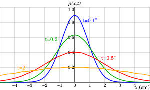
Then the density of Brownian particles ρ at point x at time t satisfies the diffusion equation:

${\displaystyle {\frac {\partial \rho }{\partial t}}=D\cdot {\frac {\partial ^{2}\rho }{\partial x^{2}}},}$

Assuming that N particles start from the origin at the initial time t = 0, the diffusion equation has the solution

${\displaystyle \rho (x,t)={\frac {N}{\sqrt {4\pi Dt}}}e^{-{\frac {x^{2}}{4Dt}}}.}$

This expression (which is a normal distribution with the mean ${\displaystyle \mu =0}$ and variance ${\displaystyle \sigma ^{2}=2Dt}$ usually called Brownian motion ${\displaystyle B_{t}}$) allowed Einstein to calculate the moments directly. The first moment is seen to vanish, meaning that the Brownian particle is equally likely to move to the left as it is to move to the right. The second moment is, however, non-vanishing, being given by

${\displaystyle {\overline {x^{2}}}=2\,D\,t.}$

This equation expresses the mean squared displacement in terms of the time elapsed and the diffusivity. From this expression Einstein argued that the displacement of a Brownian particle is not proportional to the elapsed time, but rather to its square root.^[10] His argument is based on a conceptual switch from the "ensemble" of Brownian particles to the "single" Brownian particle: we can speak of the relative number of particles at a single instant just as well as of the time it takes a Brownian particle to reach a given point.^[12]

The second part of Einstein's theory relates the diffusion constant to physically measurable quantities, such as the mean squared displacement of a particle in a given time interval. This result enables the experimental determination of Avogadro's number and therefore the size of molecules. Einstein analyzed a dynamic equilibrium being established between opposing forces. The beauty of his argument is that the final result does not depend upon which forces are involved in setting up the dynamic equilibrium.

In his original treatment, Einstein considered an osmotic pressure experiment, but the same conclusion can be reached in other ways.

Consider, for instance, particles suspended in a viscous fluid in a gravitational field. Gravity tends to make the particles settle, whereas diffusion acts to homogenize them, driving them into regions of smaller concentration. Under the action of gravity, a particle acquires a downward speed of v = μmg, where m is the mass of the particle, g is the acceleration due to gravity, and μ is the particle's mobility in the fluid. George Stokes had shown that the mobility for a spherical particle with radius r is ${\displaystyle \mu ={\tfrac {1}{6\pi \eta r}}}$, where η is the dynamic viscosity of the fluid. In a state of dynamic equilibrium, and under the hypothesis of isothermal fluid, the particles are distributed according to the barometric distribution

${\displaystyle \rho =\rho _{o}\,e^{-{\frac {m\,g\,h}{k_{\rm {B}}\,T}}},}$

where ρ − ρ_o is the difference in density of particles separated by a height difference, of ${\displaystyle h=z-z_{o}}$ , k_B is the Boltzmann constant (the ratio of the universal gas constant, R, to the Avogadro constant, N_A), and T is the absolute temperature.

The equilibrium distribution for particles of gamboge shows the tendency for granules to move to regions of lower concentration when affected by gravity.

Dynamic equilibrium is established because the more that particles are pulled down by gravity, the greater the tendency for the particles to migrate to regions of lower concentration. The flux is given by Fick's law,

${\displaystyle J=-D{\frac {d\rho }{dh}},}$

where J = ρv. Introducing the formula for ρ, we find that

${\displaystyle v={\frac {Dmg}{k_{\rm {B}}T}}.}$

In a state of dynamical equilibrium, this speed must also be equal to v = μmg. Both expressions for v are proportional to mg, reflecting that the derivation is independent of the type of forces considered. Similarly, one can derive an equivalent formula for identical charged particles of charge q in a uniform electric field of magnitude E, where mg is replaced with the electrostatic force qE. Equating these two expressions yields a formula for the diffusivity, independent of mg or qE or other such forces:

${\displaystyle {\frac {\overline {x^{2}}}{2t}}=D=\mu k_{\rm {B}}T={\frac {\mu RT}{N_{\text{A}}}}={\frac {RT}{6\pi \eta rN_{\text{A}}}}.}$

Here the first equality follows from the first part of Einstein's theory, the third equality follows from the definition of Boltzmann's constant as k_B = R / N_A, and the fourth equality follows from Stokes's formula for the mobility. By measuring the mean squared displacement over a time interval along with the universal gas constant R, the temperature T, the viscosity η, and the particle radius r, the Avogadro constant N_A can be determined.

The type of dynamical equilibrium proposed by Einstein was not new. It had been pointed out previously by J. J. Thomson^[13] in his series of lectures at Yale University in May 1903 that the dynamic equilibrium between the velocity generated by a concentration gradient given by Fick's law and the velocity due to the variation of the partial pressure caused when ions are set in motion "gives us a method of determining Avogadro's Constant which is independent of any hypothesis as to the shape or size of molecules, or of the way in which they act upon each other".^[13]

An identical expression to Einstein's formula for the diffusion coefficient was also found by Walther Nernst in 1888^[14] in which he expressed the diffusion coefficient as the ratio of the osmotic pressure to the ratio of the frictional force and the velocity to which it gives rise. The former was equated to the law of van 't Hoff while the latter was given by Stokes's law. He writes ${\displaystyle k'=p_{o}/k}$ for the diffusion coefficient k', where ${\displaystyle p_{o}}$ is the osmotic pressure and k is the ratio of the frictional force to the molecular viscosity which he assumes is given by Stokes's formula for the viscosity. Introducing the ideal gas law per unit volume for the osmotic pressure, the formula becomes identical to that of Einstein's.^[15] The use of Stokes's law in Nernst's case, as well as in Einstein and Smoluchowski, is not strictly applicable since it does not apply to the case where the radius of the sphere is small in comparison with the mean free path.^[16]

At first, the predictions of Einstein's formula were seemingly refuted by a series of experiments by Svedberg in 1906 and 1907, which gave displacements of the particles as 4 to 6 times the predicted value, and by Henri in 1908 who found displacements 3 times greater than Einstein's formula predicted.^[17] But Einstein's predictions were finally confirmed in a series of experiments carried out by Chaudesaigues in 1908 and Perrin in 1909. The confirmation of Einstein's theory constituted empirical progress for the kinetic theory of heat. In essence, Einstein showed that the motion can be predicted directly from the kinetic model of thermal equilibrium. The importance of the theory lay in the fact that it confirmed the kinetic theory's account of the second law of thermodynamics as being an essentially statistical law.^[18]

Smoluchowski model[]

Smoluchowski's theory of Brownian motion^[19] starts from the same premise as that of Einstein and derives the same probability distribution ρ(x, t) for the displacement of a Brownian particle along the x in time t. He therefore gets the same expression for the mean squared displacement: ${\displaystyle {\overline {(\Delta x)^{2}}}}$. However, when he relates it to a particle of mass m moving at a velocity ${\displaystyle u}$ which is the result of a frictional force governed by Stokes's law, he finds

${\displaystyle {\overline {(\Delta x)^{2}}}=2Dt=t{\frac {32}{81}}{\frac {u^{2}}{\pi \mu a}}=t{\frac {64}{27}}{\frac {{\frac {1}{2}}u^{2}}{3\pi \mu a}},}$

where μ is the viscosity coefficient, and ${\displaystyle a}$ is the radius of the particle. Associating the kinetic energy ${\displaystyle u^{2}/2}$ with the thermal energy RT/N, the expression for the mean squared displacement is 64/27 times that found by Einstein. The fraction 27/64 was commented on by Arnold Sommerfeld in his necrology on Smoluchowski: "The numerical coefficient of Einstein, which differs from Smoluchowski by 27/64 can only be put in doubt."^[20]

Smoluchowski^[21] attempts to answer the question of why a Brownian particle should be displaced by bombardments of smaller particles when the probabilities for striking it in the forward and rear directions are equal. If the probability of m gains and n − m losses follows a binomial distribution,

${\displaystyle P_{m,n}={\binom {n}{m}}2^{-n},}$

with equal a priori probabilities of 1/2, the mean total gain is

${\displaystyle {\overline {2m-n}}=\sum _{m={\frac {n}{2}}}^{n}(2m-n)P_{m,n}={\frac {nn!}{2^{n}\left[\left({\frac {n}{2}}\right)!\right]^{2}}}.}$

If n is large enough so that Stirling's approximation can be used in the form

${\displaystyle n!\approx \left({\frac {n}{e}}\right)^{n}{\sqrt {2\pi n}},}$

then the expected total gain will be^{[citation needed]}

${\displaystyle {\overline {2m-n}}\approx {\sqrt {\frac {2n}{\pi }}},}$

showing that it increases as the square root of the total population.

Suppose that a Brownian particle of mass M is surrounded by lighter particles of mass m which are traveling at a speed u. Then, reasons Smoluchowski, in any collision between a surrounding and Brownian particles, the velocity transmitted to the latter will be mu/M. This ratio is of the order of 10⁻⁷ cm/s. But we also have to take into consideration that in a gas there will be more than 10¹⁶ collisions in a second, and even greater in a liquid where we expect that there will be 10²⁰ collision in one second. Some of these collisions will tend to accelerate the Brownian particle; others will tend to decelerate it. If there is a mean excess of one kind of collision or the other to be of the order of 10⁸ to 10¹⁰ collisions in one second, then velocity of the Brownian particle may be anywhere between 10 and 1000 cm/s. Thus, even though there are equal probabilities for forward and backward collisions there will be a net tendency to keep the Brownian particle in motion, just as the ballot theorem predicts.

These orders of magnitude are not exact because they don't take into consideration the velocity of the Brownian particle, U, which depends on the collisions that tend to accelerate and decelerate it. The larger U is, the greater will be the collisions that will retard it so that the velocity of a Brownian particle can never increase without limit. Could such a process occur, it would be tantamount to a perpetual motion of the second type. And since equipartition of energy applies, the kinetic energy of the Brownian particle, ${\displaystyle MU^{2}/2}$, will be equal, on the average, to the kinetic energy of the surrounding fluid particle, ${\displaystyle mu^{2}/2}$.

In 1906 Smoluchowski published a one-dimensional model to describe a particle undergoing Brownian motion.^[22] The model assumes collisions with M ≫ m where M is the test particle's mass and m the mass of one of the individual particles composing the fluid. It is assumed that the particle collisions are confined to one dimension and that it is equally probable for the test particle to be hit from the left as from the right. It is also assumed that every collision always imparts the same magnitude of ΔV. If N_R is the number of collisions from the right and N_L the number of collisions from the left then after N collisions the particle's velocity will have changed by ΔV(2N_R − N). The multiplicity is then simply given by:

${\displaystyle {\binom {N}{N_{\rm {R}}}}={\frac {N!}{N_{\rm {R}}!(N-N_{\rm {R}})!}}}$

and the total number of possible states is given by 2^N. Therefore, the probability of the particle being hit from the right N_R times is:

${\displaystyle P_{N}(N_{\rm {R}})={\frac {N!}{2^{N}N_{\rm {R}}!(N-N_{\rm {R}})!}}}$

As a result of its simplicity, Smoluchowski's 1D model can only qualitatively describe Brownian motion. For a realistic particle undergoing Brownian motion in a fluid, many of the assumptions don't apply. For example, the assumption that on average occurs an equal number of collisions from the right as from the left falls apart once the particle is in motion. Also, there would be a distribution of different possible ΔVs instead of always just one in a realistic situation.

Other physics models using partial differential equations[]

The diffusion equation yields an approximation of the time evolution of the probability density function associated to the position of the particle going under a Brownian movement under the physical definition. The approximation is valid on short timescales.

The time evolution of the position of the Brownian particle itself is best described using Langevin equation, an equation which involves a random force field representing the effect of the thermal fluctuations of the solvent on the particle.

The displacement of a particle undergoing Brownian motion is obtained by solving the diffusion equation under appropriate boundary conditions and finding the rms of the solution. This shows that the displacement varies as the square root of the time (not linearly), which explains why previous experimental results concerning the velocity of Brownian particles gave nonsensical results. A linear time dependence was incorrectly assumed.

At very short time scales, however, the motion of a particle is dominated by its inertia and its displacement will be linearly dependent on time: Δx = vΔt. So the instantaneous velocity of the Brownian motion can be measured as v = Δx/Δt, when Δt << τ, where τ is the momentum relaxation time. In 2010, the instantaneous velocity of a Brownian particle (a glass microsphere trapped in air with optical tweezers) was measured successfully.^[23] The velocity data verified the Maxwell–Boltzmann velocity distribution, and the equipartition theorem for a Brownian particle.

Astrophysics: star motion within galaxies[]

In stellar dynamics, a massive body (star, black hole, etc.) can experience Brownian motion as it responds to gravitational forces from surrounding stars.^[24] The rms velocity V of the massive object, of mass M, is related to the rms velocity ${\displaystyle v_{\star }}$ of the background stars by

${\displaystyle MV^{2}\approx mv_{\star }^{2}}$

where ${\displaystyle m\ll M}$ is the mass of the background stars. The gravitational force from the massive object causes nearby stars to move faster than they otherwise would, increasing both ${\displaystyle v_{\star }}$ and V.^[24] The Brownian velocity of Sgr A*, the supermassive black hole at the center of the Milky Way galaxy, is predicted from this formula to be less than 1 km s⁻¹.^[25]

Mathematics[]

Play media

An animated example of a Brownian motion-like random walk on a torus. In the scaling limit, random walk approaches the Wiener process according to Donsker's theorem.

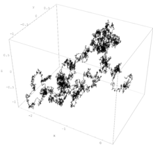
In mathematics, Brownian motion is described by the Wiener process, a continuous-time stochastic process named in honor of Norbert Wiener. It is one of the best known Lévy processes (càdlàg stochastic processes with stationary independent increments) and occurs frequently in pure and applied mathematics, economics and physics.

A single realisation of three-dimensional Brownian motion for times 0 ≤ t ≤ 2

The Wiener process W_t is characterized by four facts:^{[citation needed]}

1. W₀ = 0
2. W_t is almost surely continuous
3. W_t has independent increments
4. ${\displaystyle W_{t}-W_{s}\sim {\mathcal {N}}(0,t-s)}$ (for ${\displaystyle 0\leq s\leq t}$).

${\displaystyle {\mathcal {N}}(\mu ,\sigma ^{2})}$ denotes the normal distribution with expected value μ and variance σ². The condition that it has independent increments means that if ${\displaystyle 0\leq s_{1}<t_{1}\leq s_{2}<t_{2}}$ then ${\displaystyle W_{t_{1}}-W_{s_{1}}}$ and ${\displaystyle W_{t_{2}}-W_{s_{2}}}$ are independent random variables.

An alternative characterisation of the Wiener process is the so-called Lévy characterisation that says that the Wiener process is an almost surely continuous martingale with W₀ = 0 and quadratic variation ${\displaystyle [W_{t},W_{t}]=t}$.

A third characterisation is that the Wiener process has a spectral representation as a sine series whose coefficients are independent ${\displaystyle {\mathcal {N}}(0,1)}$ random variables. This representation can be obtained using the Karhunen–Loève theorem.

The Wiener process can be constructed as the scaling limit of a random walk, or other discrete-time stochastic processes with stationary independent increments. This is known as Donsker's theorem. Like the random walk, the Wiener process is recurrent in one or two dimensions (meaning that it returns almost surely to any fixed neighborhood of the origin infinitely often) whereas it is not recurrent in dimensions three and higher. Unlike the random walk, it is scale invariant.

The time evolution of the position of the Brownian particle itself can be described approximately by a Langevin equation, an equation which involves a random force field representing the effect of the thermal fluctuations of the solvent on the Brownian particle. On long timescales, the mathematical Brownian motion is well described by a Langevin equation. On small timescales, inertial effects are prevalent in the Langevin equation. However the mathematical Brownian motion is exempt of such inertial effects. Inertial effects have to be considered in the Langevin equation, otherwise the equation becomes singular.^{[clarification needed]} so that simply removing the inertia term from this equation would not yield an exact description, but rather a singular behavior in which the particle doesn't move at all.^{[clarification needed]}

Statistics[]

The Brownian motion can be modeled by a random walk.^[26] Random walks in porous media or fractals are anomalous.^[27]

In the general case, Brownian motion is a non-Markov random process and described by stochastic integral equations.^[28]

Lévy characterisation[]

The French mathematician Paul Lévy proved the following theorem, which gives a necessary and sufficient condition for a continuous Rⁿ-valued stochastic process X to actually be n-dimensional Brownian motion. Hence, Lévy's condition can actually be used as an alternative definition of Brownian motion.

Let X = (X₁, ..., X_n) be a continuous stochastic process on a probability space (Ω, Σ, P) taking values in Rⁿ. Then the following are equivalent:

1. X is a Brownian motion with respect to P, i.e., the law of X with respect to P is the same as the law of an n-dimensional Brownian motion, i.e., the push-forward measure X_∗(P) is classical Wiener measure on C₀([0, +∞); Rⁿ).
2. both
   1. X is a martingale with respect to P (and its own natural filtration); and
   2. for all 1 ≤ i, j ≤ n, X_i(t)X_j(t) −δ_ijt is a martingale with respect to P (and its own natural filtration), where δ_ij denotes the Kronecker delta.

Spectral content[]

The spectral content of a stochastic process ${\displaystyle X_{t}}$ can be found from the power spectral density, formally defined as

${\displaystyle S(\omega )=\lim _{T\to \infty }{\frac {1}{T}}\mathbb {E} \left\{\left|\int _{0}^{T}e^{i\omega t}X_{t}dt\right|^{2}\right\}}$,

where ${\displaystyle \mathbb {E} }$ stands for the expected value. The power spectral density of Brownian motion is found to be^[29]

${\displaystyle S_{BM}(\omega )={\frac {4D}{\omega ^{2}}}}$.

where ${\displaystyle D}$ is the diffusion coefficient of ${\displaystyle X_{t}}$. For naturally occurring signals, the spectral content can be found from the power spectral density of a single realization, with finite available time, i.e.,

${\displaystyle S^{(1)}(\omega ,T)={\frac {1}{T}}\left|\int _{0}^{T}e^{i\omega t}X_{t}dt\right|^{2}}$,

which for an individual realization of a Brownian motion trajectory,^[30] it is found to have expected value ${\displaystyle \mu _{BM}(\omega ,T)}$

${\displaystyle \mu _{BM}(\omega ,T)={\frac {4D}{\omega ^{2}}}\left[1-{\frac {\sin \left(\omega T\right)}{\omega T}}\right]}$

and variance ${\displaystyle \sigma _{BM}^{2}(\omega ,T)}$^[30]

${\displaystyle \sigma _{S}^{2}(f,T)=\mathbb {E} \left\{\left(S_{T}^{(j)}(f)\right)^{2}\right\}-\mu _{S}^{2}(f,T)={\frac {20D^{2}}{f^{4}}}{\Bigg [}1-{\Big (}6-\cos \left(fT\right){\Big )}{\frac {2\sin \left(fT\right)}{5fT}}+{\frac {{\Big (}17-\cos \left(2fT\right)-16\cos \left(fT\right){\Big )}}{10f^{2}T^{2}}}{\Bigg ]}}$.

For sufficiently long realization times, the expected value of the power spectrum of a single trajectory converges to the formally defined power spectral density ${\displaystyle S(\omega )}$, but its coefficient of variation ${\displaystyle \gamma ={\sqrt {\sigma ^{2}}}/\mu }$ tends to ${\displaystyle {\sqrt {5}}/2}$. This implies the distribution of ${\displaystyle S^{(1)}(\omega ,T)}$ is broad even in the infinite time limit.

Riemannian manifold[]

Brownian motion on a sphere

This section may be too technical for most readers to understand. Please to make it understandable to non-experts, without removing the technical details. (June 2011) (Learn how and when to remove this template message)

The infinitesimal generator (and hence characteristic operator) of a Brownian motion on Rⁿ is easily calculated to be ½Δ, where Δ denotes the Laplace operator. In image processing and computer vision, the Laplacian operator has been used for various tasks such as blob and edge detection. This observation is useful in defining Brownian motion on an m-dimensional Riemannian manifold (M, g): a Brownian motion on M is defined to be a diffusion on M whose characteristic operator ${\displaystyle {\mathcal {A}}}$ in local coordinates x_i, 1 ≤ i ≤ m, is given by ½Δ_LB, where Δ_LB is the Laplace–Beltrami operator given in local coordinates by

${\displaystyle \Delta _{\mathrm {LB} }={\frac {1}{\sqrt {\det(g)}}}\sum _{i=1}^{m}{\frac {\partial }{\partial x_{i}}}\left({\sqrt {\det(g)}}\sum _{j=1}^{m}g^{ij}{\frac {\partial }{\partial x_{j}}}\right),}$

where [g^ij] = [g_ij]⁻¹ in the sense of the inverse of a square matrix.

Narrow escape[]

The narrow escape problem is a ubiquitous problem in biology, biophysics and cellular biology which has the following formulation: a Brownian particle (ion, molecule, or protein) is confined to a bounded domain (a compartment or a cell) by a reflecting boundary, except for a small window through which it can escape. The narrow escape problem is that of calculating the mean escape time. This time diverges as the window shrinks, thus rendering the calculation a singular perturbation problem.

See also[]

References[]

Further reading[]

• Brown, Robert (1828). "A brief account of microscopical observations made in the months of June, July and August, 1827, on the particles contained in the pollen of plants; and on the general existence of active molecules in organic and inorganic bodies" (PDF). Philosophical Magazine. 4 (21): 161–173. doi:10.1080/14786442808674769. Also includes a subsequent defense by Brown of his original observations, Additional remarks on active molecules.
• Chaudesaigues, M. (1908). "Le mouvement brownien et la formule d'Einstein" [Brownian motion and Einstein's formula]. Comptes Rendus (in French). 147: 1044–6.
• Clark, P. (1976). "Atomism versus thermodynamics". In Howson, Colin (ed.). Method and appraisal in the physical sciences. Cambridge University Press. ISBN 978-0521211109.
• Cohen, Ruben D. (1986). "Self Similarity in Brownian Motion and Other Ergodic Phenomena" (PDF). Journal of Chemical Education. 63 (11): 933–934. Bibcode:1986JChEd..63..933C. doi:10.1021/ed063p933.
• Dubins, Lester E.; Schwarz, Gideon (15 May 1965). "On Continuous Martingales". Proceedings of the National Academy of Sciences of the United States of America. 53 (3): 913–916. Bibcode:1965PNAS...53..913D. doi:10.1073/pnas.53.5.913. JSTOR 72837. PMC 301348. PMID 16591279.
• Einstein, A. (1956). Investigations on the Theory of Brownian Movement. New York: Dover. ISBN 978-0-486-60304-9. Retrieved 6 January 2014.
• Henri, V. (1908). "Études cinématographique du mouvement brownien" [Cinematographic studies of Brownian motion]. Comptes Rendus (in French) (146): 1024–6.
• Lucretius, On The Nature of Things, translated by William Ellery Leonard. (on-line version, from Project Gutenberg. See the heading 'Atomic Motions'; this translation differs slightly from the one quoted).
• Nelson, Edward, (1967). Dynamical Theories of Brownian Motion. (PDF version of this out-of-print book, from the author's webpage.) This is primarily a mathematical work, but the first four chapters discuss the history of the topic, in the era from Brown to Einstein.
• Pearle, P.; Collett, B.; Bart, K.; Bilderback, D.; Newman, D.; Samuels, S. (2010). "What Brown saw and you can too". American Journal of Physics. 78 (12): 1278–1289. arXiv:1008.0039. Bibcode:2010AmJPh..78.1278P. doi:10.1119/1.3475685. S2CID 12342287.
• Perrin, J. (1909). "Mouvement brownien et réalité moléculaire" [Brownian movement and molecular reality]. Annales de chimie et de physique. 8th series. 18: 5–114.
  • See also Perrin's book "Les Atomes" (1914).
• von Smoluchowski, M. (1906). "Zur kinetischen Theorie der Brownschen Molekularbewegung und der Suspensionen". Annalen der Physik. 21 (14): 756–780. Bibcode:1906AnP...326..756V. doi:10.1002/andp.19063261405.
• Svedberg, T. (1907). Studien zur Lehre von den kolloiden Losungen.
• Theile, T. N.
  • Danish version: "Om Anvendelse af mindste Kvadraters Methode i nogle Tilfælde, hvor en Komplikation af visse Slags uensartede tilfældige Fejlkilder giver Fejlene en 'systematisk' Karakter".
  • French version: "Sur la compensation de quelques erreurs quasi-systématiques par la méthodes de moindre carrés" published simultaneously in Vidensk. Selsk. Skr. 5. Rk., naturvid. og mat. Afd., 12:381–408, 1880.

External links[]

Wikimedia Commons has media related to Brownian motion.

Wikisource has original text related to this article: A brief account of microscopical observations made on the particles contained in the pollen of plants

• Einstein on Brownian Motion
• Discusses history, botany and physics of Brown's original observations, with videos
• "Einstein's prediction finally witnessed one century later" : a test to observe the velocity of Brownian motion
• Large-Scale Brownian Motion Demonstration^{[permanent dead link]}