Digital image processing
Digital image processing is the use of a digital computer to process digital images through an algorithm.[1][2] As a subcategory or field of digital signal processing, digital image processing has many advantages over analog image processing. It allows a much wider range of algorithms to be applied to the input data and can avoid problems such as the build-up of noise and distortion during processing. Since images are defined over two dimensions (perhaps more) digital image processing may be modeled in the form of multidimensional systems. The generation and development of digital image processing are mainly affected by three factors: first, the development of computers; second, the development of mathematics (especially the creation and improvement of discrete mathematics theory); third, the demand for a wide range of applications in environment, agriculture, military, industry and medical science has increased.
History[]
Many of the techniques of digital image processing, or digital picture processing as it often was called, were developed in the 1960s, at Bell Laboratories, the Jet Propulsion Laboratory, Massachusetts Institute of Technology, University of Maryland, and a few other research facilities, with application to satellite imagery, wire-photo standards conversion, medical imaging, videophone, character recognition, and photograph enhancement.[3] The purpose of early image processing was to improve the quality of the image. It was aimed for human beings to improve the visual effect of people. In image processing, the input is a low-quality image, and the output is an image with improved quality. Common image processing include image enhancement, restoration, encoding, and compression. The first successful application was the American Jet Propulsion Laboratory (JPL). They used image processing techniques such as geometric correction, gradation transformation, noise removal, etc. on the thousands of lunar photos sent back by the Space Detector Ranger 7 in 1964, taking into account the position of the sun and the environment of the moon. The impact of the successful mapping of the moon's surface map by the computer has been a huge success. Later, more complex image processing was performed on the nearly 100,000 photos sent back by the spacecraft, so that the topographic map, color map and panoramic mosaic of the moon were obtained, which achieved extraordinary results and laid a solid foundation for human landing on the moon.[4]
The cost of processing was fairly high, however, with the computing equipment of that era. That changed in the 1970s, when digital image processing proliferated as cheaper computers and dedicated hardware became available. This led to images being processed in real-time, for some dedicated problems such as television standards conversion. As general-purpose computers became faster, they started to take over the role of dedicated hardware for all but the most specialized and computer-intensive operations. With the fast computers and signal processors available in the 2000s, digital image processing has become the most common form of image processing, and is generally used because it is not only the most versatile method, but also the cheapest.
Image sensors[]
The basis for modern image sensors is metal-oxide-semiconductor (MOS) technology,[5] which originates from the invention of the MOSFET (MOS field-effect transistor) by Mohamed M. Atalla and Dawon Kahng at Bell Labs in 1959.[6] This led to the development of digital semiconductor image sensors, including the charge-coupled device (CCD) and later the CMOS sensor.[5]
The charge-coupled device was invented by Willard S. Boyle and George E. Smith at Bell Labs in 1969.[7] While researching MOS technology, they realized that an electric charge was the analogy of the magnetic bubble and that it could be stored on a tiny MOS capacitor. As it was fairly straightforward to fabricate a series of MOS capacitors in a row, they connected a suitable voltage to them so that the charge could be stepped along from one to the next.[5] The CCD is a semiconductor circuit that was later used in the first digital video cameras for television broadcasting.[8]
The NMOS active-pixel sensor (APS) was invented by Olympus in Japan during the mid-1980s. This was enabled by advances in MOS semiconductor device fabrication, with MOSFET scaling reaching smaller micron and then sub-micron levels.[9][10] The NMOS APS was fabricated by Tsutomu Nakamura's team at Olympus in 1985.[11] The CMOS active-pixel sensor (CMOS sensor) was later developed by Eric Fossum's team at the NASA Jet Propulsion Laboratory in 1993.[12] By 2007, sales of CMOS sensors had surpassed CCD sensors.[13]
Image compression[]
An important development in digital image compression technology was the discrete cosine transform (DCT), a lossy compression technique first proposed by Nasir Ahmed in 1972.[14] DCT compression became the basis for JPEG, which was introduced by the Joint Photographic Experts Group in 1992.[15] JPEG compresses images down to much smaller file sizes, and has become the most widely used image file format on the Internet.[16] Its highly efficient DCT compression algorithm was largely responsible for the wide proliferation of digital images and digital photos,[17] with several billion JPEG images produced every day as of 2015.[18]
Digital signal processor (DSP)[]
Electronic signal processing was revolutionized by the wide adoption of MOS technology in the 1970s.[19] MOS integrated circuit technology was the basis for the first single-chip microprocessors and microcontrollers in the early 1970s,[20] and then the first single-chip digital signal processor (DSP) chips in the late 1970s.[21][22] DSP chips have since been widely used in digital image processing.[21]
The discrete cosine transform (DCT) image compression algorithm has been widely implemented in DSP chips, with many companies developing DSP chips based on DCT technology. DCTs are widely used for encoding, decoding, video coding, audio coding, multiplexing, control signals, signaling, analog-to-digital conversion, formatting luminance and color differences, and color formats such as YUV444 and YUV411. DCTs are also used for encoding operations such as motion estimation, motion compensation, inter-frame prediction, quantization, perceptual weighting, entropy encoding, variable encoding, and motion vectors, and decoding operations such as the inverse operation between different color formats (YIQ, YUV and RGB) for display purposes. DCTs are also commonly used for high-definition television (HDTV) encoder/decoder chips.[23]
Medical imaging[]
In 1972, the engineer from British company EMI Housfield invented the X-ray computed tomography device for head diagnosis, which is what is usually called CT (computer tomography). The CT nucleus method is based on the projection of the human head section and is processed by computer to reconstruct the cross-sectional image, which is called image reconstruction. In 1975, EMI successfully developed a CT device for the whole body, which obtained a clear tomographic image of various parts of the human body. In 1979, this diagnostic technique won the Nobel Prize.[4] Digital image processing technology for medical applications was inducted into the Space Foundation Space Technology Hall of Fame in 1994.[24]
Tasks[]
Digital image processing allows the use of much more complex algorithms, and hence, can offer both more sophisticated performance at simple tasks, and the implementation of methods which would be impossible by analogue means.
In particular, digital image processing is a concrete application of, and a practical technology based on:
- Classification
- Feature extraction
- Multi-scale signal analysis
- Pattern recognition
- Projection
Some techniques which are used in digital image processing include:
- Anisotropic diffusion
- Hidden Markov models
- Image editing
- Image restoration
- Independent component analysis
- Linear filtering
- Neural networks
- Partial differential equations
- Pixelation
- Point feature matching
- Principal components analysis
- Self-organizing maps
- Wavelets
Digital image transformations[]
Filtering[]
Digital filters are used to blur and sharpen digital images. Filtering can be performed by:
- convolution with specifically designed kernels (filter array) in the spatial domain[25]
- masking specific frequency regions in the frequency (Fourier) domain
The following examples show both methods:[26]
| Filter type | Kernel or mask | Example |
|---|---|---|
| Original Image | 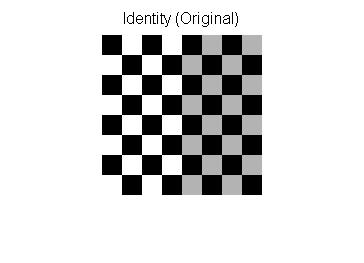
| |
| Spatial Lowpass | 
| |
| Spatial Highpass | 
| |
| Fourier Representation | Pseudo-code:
image = checkerboard F = Fourier Transform of image Show Image: log(1+Absolute Value(F)) |

|
| Fourier Lowpass | 
|
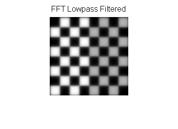
|
| Fourier Highpass | 
|

|


Image padding in Fourier domain filtering[]
Images are typically padded before being transformed to the Fourier space, the highpass filtered images below illustrate the consequences of different padding techniques:
| Zero padded | Repeated edge padded |
|---|---|
|
|

|
Notice that the highpass filter shows extra edges when zero padded compared to the repeated edge padding.
Filtering code examples[]
MATLAB example for spatial domain highpass filtering.
img=checkerboard(20);                           % generate checkerboard
% **************************  SPATIAL DOMAIN  ***************************
klaplace=[0 -1 0; -1 5 -1;  0 -1 0];             % Laplacian filter kernel
X=conv2(img,klaplace);                          % convolve test img with
                                                % 3x3 Laplacian kernel
figure()
imshow(X,[])                                    % show Laplacian filtered
title('Laplacian Edge Detection')
Affine transformations[]
Affine transformations enable basic image transformations including scale, rotate, translate, mirror and shear as is shown in the following examples:[26]
| Transformation Name | Affine Matrix | Example |
|---|---|---|
| Identity | 
| |
| Reflection | 
| |
| Scale | 
| |
| Rotate |  where θ = π/6 =30° where θ = π/6 =30°
| |
| Shear | 
|


To apply the affine matrix to an image, the image is converted to matrix in which each entry corresponds to the pixel intensity at that location. Then each pixel's location can be represented as a vector indicating the coordinates of that pixel in the image, [x, y], where x and y are the row and column of a pixel in the image matrix. This allows the coordinate to be multiplied by an affine-transformation matrix, which gives the position that the pixel value will be copied to in the output image.
However, to allow transformations that require translation transformations, 3 dimensional homogeneous coordinates are needed. The third dimension is usually set to a non-zero constant, usually 1, so that the new coordinate is [x, y, 1]. This allows the coordinate vector to be multiplied by a 3 by 3 matrix, enabling translation shifts. So the third dimension, which is the constant 1, allows translation.
Because matrix multiplication is associative, multiple affine transformations can be combined into a single affine transformation by multiplying the matrix of each individual transformation in the order that the transformations are done. This results in a single matrix that, when applied to a point vector, gives the same result as all the individual transformations performed on the vector [x, y, 1] in sequence. Thus a sequence of affine transformation matrices can be reduced to a single affine transformation matrix.
For example, 2 dimensional coordinates only allow rotation about the origin (0, 0). But 3 dimensional homogeneous coordinates can be used to first translate any point to (0, 0), then perform the rotation, and lastly translate the origin (0, 0) back to the original point (the opposite of the first translation). These 3 affine transformations can be combined into a single matrix, thus allowing rotation around any point in the image.[27]
Image denoising with Morphology[]
Mathematical morphology is suitable for denoising images. Structuring element are important in Mathematical morphology.
The following examples are about Structuring elements. The denoise function, image as I, and structuring element as B are shown as below and table.
eg.

Define Dilation(I, B)(i,j) = . Let Dilation(I,B) = D(I,B)

D(I', B)(1,1) =

Define Erosion(I, B)(i,j) = . Let Erosion(I,B) = E(I,B)

E(I', B)(1,1) =

After dilation After erosion


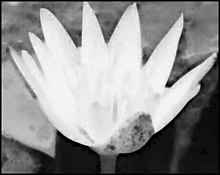
An opening method is just simply erosion first, and then dilation while the closing method is vice versa. In reality, the D(I,B) and E(I,B) can implemented by Convolution
| Structuring element | Mask | Code | Example |
|---|---|---|---|
| Original Image | None | Use Matlab to read Original image
original = imread('scene.jpg');
image = rgb2gray(original);
[r, c, channel] = size(image);
se = logical([1 1 1 ; 1 1 1 ; 1 1 1]);
[p, q] = size(se);
halfH = floor(p/2);
halfW = floor(q/2);
time = 3;           % denoising 3 times with all method
|
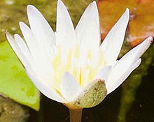 original lotus |
| Dilation | Use Matlab to dilation
imwrite(image, "scene_dil.jpg")
extractmax = zeros(size(image), class(image));
for i = 1 : time
    dil_image = imread('scene_dil.jpg');
    for col = (halfW + 1): (c - halfW)
        for row = (halfH + 1) : (r - halfH)
            dpointD = row - halfH;
            dpointU = row + halfH;
            dpointL = col - halfW;
            dpointR = col + halfW;
            dneighbor = dil_image(dpointD:dpointU, dpointL:dpointR);
            filter = dneighbor(se);
            extractmax(row, col) = max(filter);
        end
    end
    imwrite(extractmax, "scene_dil.jpg");
end
|
 denoising picture with dilation method | |
| Erosion | Use Matlab to erosion
imwrite(image, 'scene_ero.jpg');
extractmin = zeros(size(image), class(image));
for i = 1: time
    ero_image = imread('scene_ero.jpg');
    for col = (halfW + 1): (c - halfW)
        for row = (halfH +1): (r -halfH)
            pointDown = row-halfH;
            pointUp = row+halfH;
            pointLeft = col-halfW;
            pointRight = col+halfW;
            neighbor = ero_image(pointDown:pointUp,pointLeft:pointRight);
            filter = neighbor(se);
            extractmin(row, col) = min(filter);
        end
    end
    imwrite(extractmin, "scene_ero.jpg");
end
|
 | |
| Opening | Use Matlab to Opening
imwrite(extractmin, "scene_opening.jpg")
extractopen = zeros(size(image), class(image));
for i = 1 : time
    dil_image = imread('scene_opening.jpg');
    for col = (halfW + 1): (c - halfW)
        for row = (halfH + 1) : (r - halfH)
            dpointD = row - halfH;
            dpointU = row + halfH;
            dpointL = col - halfW;
            dpointR = col + halfW;
            dneighbor = dil_image(dpointD:dpointU, dpointL:dpointR);
            filter = dneighbor(se);
            extractopen(row, col) = max(filter);
        end
    end
    imwrite(extractopen, "scene_opening.jpg");
end
|
 | |
| Closing | Use Matlab to Closing
imwrite(extractmax, "scene_closing.jpg")
extractclose = zeros(size(image), class(image));
for i = 1 : time
    ero_image = imread('scene_closing.jpg');
    for col = (halfW + 1): (c - halfW)
        for row = (halfH + 1) : (r - halfH)
            dpointD = row - halfH;
            dpointU = row + halfH;
            dpointL = col - halfW;
            dpointR = col + halfW;
            dneighbor = ero_image(dpointD:dpointU, dpointL:dpointR);
            filter = dneighbor(se);
            extractclose(row, col) = min(filter);
        end
    end
    imwrite(extractclose, "scene_closing.jpg");
end
|
 denoising picture with closing method |

In order to apply the denoising method to an image, the image is converted into grayscale. A mask with denoising method is logical matrix with . The denoising methods start from the center of the picture with half of height, half of width, and end with the image boundary of row number, column number. Neighbor is a block in the original image with the boundary [the point below center: the point above, the point on left of center: the point on the right of center]. Convolution Neighbor and structuring element and then replace the center with a minimum of neighbor.
![{\displaystyle [111;111;111]}](https://wikimedia.org/api/rest_v1/media/math/render/svg/942ebdef22e25cc555f1fb3dc7ec026a46e95fb2)
Take the Closing method for example.
Dilation first
- Read the image and convert it into grayscale with Matlab.
- Get the size of an image. The return value row numbers and column numbers are the boundaries we are going to use later.
- structuring elements depend on your dilation or erosion function. The minimum of the neighbor of a pixel leads to an erosion method and the maximum of neighbor leads to a dilation method.
- Set the time for dilation, erosion, and closing.
- Create a zero matrix of the same size as the original image.
- Dilation first with structuring window.
- structuring window is 3*3 matrix and convolution
- For loop extract the minimum with window from row range [2 ~ image height - 1] with column range [2 ~ image width - 1]
- Fill the minimum value to the zero matrix and save a new image
- For the boundary, it can still be improved. Since in the method, a boundary is ignored. Padding elements can be applied to deal with boundaries.
Then Erosion (Take the dilation image as input)
- Create a zero matrix of the same size as the original image.
- Erosion with structuring window.
- structuring window is 3*3 matrix and convolution
- For loop extract the maximum with window from row range [2 ~ image height - 1] with column range [2 ~ image width - 1]
- Fill the maximum value to the zero matrix and save a new image
- For the boundary, it can still be improved. Since in the method, boundary is ignored. Padding elements can be applied to deal with boundaries.
- Results are as above table shown
Applications[]
Digital camera images[]
Digital cameras generally include specialized digital image processing hardware – either dedicated chips or added circuitry on other chips – to convert the raw data from their image sensor into a color-corrected image in a standard image file format.
Film[]
Westworld (1973) was the first feature film to use the digital image processing to pixellate photography to simulate an android's point of view.[28]
Face detection[]

Face detection can be implemented with Mathematical morphology, Discrete cosine transform which is usually called DCT, and horizontal Projection (mathematics).
General method with feature-based method
The feature-based method of face detection is using skin tone, edge detection, face shape, and feature of a face (like eyes, mouse, and etc) to achieve face detection. The skin tone, face shape, and all the unique elements that only the human face have can be described as features.
Process explanation
- Given a batch of face images, first, extract the skin tone range by sampling face images. The skin tone range is just a skin filter.
- Structural similarity index measure (SSIM) can be applied to compare images in terms of extracting the skin tone.
- Normally, HSV or RGB color spaces are suitable for the skin filter. Eg. HSV mode, the skin tone range is [0,48,50] ~ [20,255,255]
- After filtering images with skin tone, to get the face edge, morphology and DCT are used to remove noise and fill up missing skin areas.
- Opening method or closing method can be used to achieve filling up missing skin.
- DCT is to avoid the object with tone-like skin. Since human faces always have higher texture.
- Sobel operator or other operators can be applied to detect face edge.
- To position human features like eyes, using the projection and find the peak of the histogram of projection help to get the detail feature like mouse, hair, and lip.
- Projection is just projecting the image to see the high frequency which is usually the feature position.
Improvement of image quality method[]
Image quality can be influenced by camera vibration, over-exposure, gray level distribution too centralized, and noise, etc. For example, noise problem can be solved by Smoothing method while gray level distribution problem can be improved by Histogram Equalization.
Smoothing method
In drawing, if there is some dissatisfied color, taking some color around dissatisfied color and averaging them. This is an easy way to think of Smoothing method.
Smoothing method can be implemented with mask and Convolution. Take the small image and mask for instance as below.
image is

mask is

After Convolution and smoothing, image is

Oberseving image[1, 1], image[1, 2], image[2, 1], and image[2, 2].
The original image pixel is 1, 4, 28, 30. After smoothing mask, the pixel becomes 9, 10, 9, 9 respectively.
new image[1, 1] = * (image[0,0]+image[0,1]+image[0,2]+image[1,0]+image[1,1]+image[1,2]+image[2,0]+image[2,1]+image[2,2])

new image[1, 1] = floor( * (2+5+6+3+1+4+1+28+30)) = 9
new image[1, 2] = floor({ * (5+6+5+1+4+6+28+30+2)) = 10
new image[2, 1] = floor( * (3+1+4+1+28+30+73+3+2)) = 9
new image[2, 2] = floor( * (1+4+6+28+30+2+3+2+2)) = 9
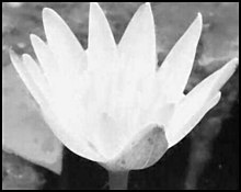
Gray Level Histogram method
Generally, given a gray level histogram from an image as below. Changing the histogram to uniform distribution from an image is usually what we called Histogram equalization.

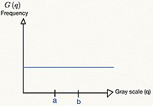
In discrete time, the area of gray level histogram is (see figure 1) while the area of uniform distribution is (see figure 2). It's clear that the area won't change, so .


From the uniform distribution, the probability of is while the


In continuous time, the equation is .

Moreover, based on the definition of a function, the Gray level histogram method is like finding a function that satisfies f(p)=q.

| Improvement method | Issue | Before improvement | Process | After improvement |
|---|---|---|---|---|
| Smoothing method | noise
with Matlab, salt & pepper with 0.01 parameter is added |
 |
|
 |
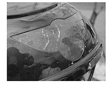
| Histogram Equalization | Gray level distribution too centralized | 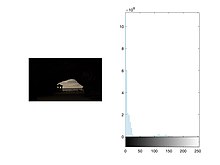 |
Refer to the Histogram equalization | 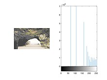 |
Fatigue detection and monitoring technologies[]
There were significant advancements in fatigue monitoring technology the past decade. These innovative technology solutions are now commercially available and offer real safety benefits to drivers, operators and other shift workers across all industries.[29]
Software developers, engineers and scientists develop fatigue detection software using various physiological cues to determine the state of fatigue or drowsiness. The measurement of brain activity (electroencephalogram) is widely accepted as the standard in fatigue monitoring. Other technology used to determine fatigue related impairment include behavioural symptom measurements such as; eye behaviour, gaze direction, micro-corrections in steering and throttle use as well as heart rate variability.[citation needed]
See also[]
- Digital imaging
- Computer graphics
- Computer vision
- CVIPtools
- Digitizing
- Free boundary condition
- GPGPU
- Homomorphic filtering
- Image analysis
- IEEE Intelligent Transportation Systems Society
- Multidimensional systems
- Remote sensing software
- Standard test image
- Superresolution
- Total variation denoising
- Machine Vision
- Bounded variation
- Radiomics
References[]
- ^ Chakravorty, Pragnan (2018). "What is a Signal? [Lecture Notes]". IEEE Signal Processing Magazine. 35 (5): 175–177. Bibcode:2018ISPM...35..175C. doi:10.1109/MSP.2018.2832195. S2CID 52164353.
- ^ Gonzalez, Rafael (2018). Digital image processing. New York, NY: Pearson. ISBN 978-0-13-335672-4. OCLC 966609831.
- ^ Azriel Rosenfeld, Picture Processing by Computer, New York: Academic Press, 1969
- ^ Jump up to: a b Gonzalez, Rafael C. (2008). Digital image processing. Woods, Richard E. (Richard Eugene), 1954- (3rd ed.). Upper Saddle River, N.J.: Prentice Hall. pp. 23–28. ISBN 9780131687288. OCLC 137312858.
- ^ Jump up to: a b c Williams, J. B. (2017). The Electronics Revolution: Inventing the Future. Springer. pp. 245–8. ISBN 9783319490885.
- ^ "1960: Metal Oxide Semiconductor (MOS) Transistor Demonstrated". The Silicon Engine. Computer History Museum. Archived from the original on 3 October 2019. Retrieved 31 August 2019.
- ^ James R. Janesick (2001). Scientific charge-coupled devices. SPIE Press. pp. 3–4. ISBN 978-0-8194-3698-6.
- ^ Boyle, William S; Smith, George E. (1970). "Charge Coupled Semiconductor Devices". Bell Syst. Tech. J. 49 (4): 587–593. doi:10.1002/j.1538-7305.1970.tb01790.x.
- ^ Fossum, Eric R. (12 July 1993). "Active pixel sensors: Are CCDS dinosaurs?". In Blouke, Morley M. (ed.). Charge-Coupled Devices and Solid State Optical Sensors III. Proceedings of the SPIE. 1900. pp. 2–14. Bibcode:1993SPIE.1900....2F. CiteSeerX 10.1.1.408.6558. doi:10.1117/12.148585. S2CID 10556755.
- ^ Fossum, Eric R. (2007). "Active Pixel Sensors". S2CID 18831792. Cite journal requires
|journal=(help) - ^ Matsumoto, Kazuya; et al. (1985). "A new MOS phototransistor operating in a non-destructive readout mode". Japanese Journal of Applied Physics. 24 (5A): L323. Bibcode:1985JaJAP..24L.323M. doi:10.1143/JJAP.24.L323.
- ^ Fossum, Eric R.; Hondongwa, D. B. (2014). "A Review of the Pinned Photodiode for CCD and CMOS Image Sensors". IEEE Journal of the Electron Devices Society. 2 (3): 33–43. doi:10.1109/JEDS.2014.2306412.
- ^ "CMOS Image Sensor Sales Stay on Record-Breaking Pace". IC Insights. 8 May 2018. Archived from the original on 21 June 2019. Retrieved 6 October 2019.
- ^ Ahmed, Nasir (January 1991). "How I Came Up With the Discrete Cosine Transform". Digital Signal Processing. 1 (1): 4–5. doi:10.1016/1051-2004(91)90086-Z. Archived from the original on 10 June 2016. Retrieved 10 October 2019.
- ^ "T.81 – DIGITAL COMPRESSION AND CODING OF CONTINUOUS-TONE STILL IMAGES – REQUIREMENTS AND GUIDELINES" (PDF). CCITT. September 1992. Archived (PDF) from the original on 17 July 2019. Retrieved 12 July 2019.
- ^ "The JPEG image format explained". BT.com. BT Group. 31 May 2018. Archived from the original on 5 August 2019. Retrieved 5 August 2019.
- ^ "What Is a JPEG? The Invisible Object You See Every Day". The Atlantic. 24 September 2013. Archived from the original on 9 October 2019. Retrieved 13 September 2019.
- ^ Baraniuk, Chris (15 October 2015). "Copy protections could come to JPEGs". BBC News. BBC. Archived from the original on 9 October 2019. Retrieved 13 September 2019.
- ^ Grant, Duncan Andrew; Gowar, John (1989). Power MOSFETS: theory and applications. Wiley. p. 1. ISBN 9780471828679.
The metal-oxide-semiconductor field-effect transistor (MOSFET) is the most commonly used active device in the very large-scale integration of digital integrated circuits (VLSI). During the 1970s these components revolutionized electronic signal processing, control systems and computers.
- ^ Shirriff, Ken (30 August 2016). "The Surprising Story of the First Microprocessors". IEEE Spectrum. Institute of Electrical and Electronics Engineers. 53 (9): 48–54. doi:10.1109/MSPEC.2016.7551353. S2CID 32003640. Archived from the original on 13 October 2019. Retrieved 13 October 2019.
- ^ Jump up to: a b "1979: Single Chip Digital Signal Processor Introduced". The Silicon Engine. Computer History Museum. Archived from the original on 3 October 2019. Retrieved 14 October 2019.
- ^ Taranovich, Steve (27 August 2012). "30 years of DSP: From a child's toy to 4G and beyond". EDN. Archived from the original on 14 October 2019. Retrieved 14 October 2019.
- ^ Stanković, Radomir S.; Astola, Jaakko T. (2012). "Reminiscences of the Early Work in DCT: Interview with K.R. Rao" (PDF). Reprints from the Early Days of Information Sciences. 60. Archived (PDF) from the original on 13 October 2019. Retrieved 13 October 2019.
- ^ "Space Technology Hall of Fame:Inducted Technologies/1994". Space Foundation. 1994. Archived from the original on 4 July 2011. Retrieved 7 January 2010.
- ^ Zhang, M. Z.; Livingston, A. R.; Asari, V. K. (2008). "A High Performance Architecture for Implementation of 2-D Convolution with Quadrant Symmetric Kernels". International Journal of Computers and Applications. 30 (4): 298–308. doi:10.1080/1206212x.2008.11441909. S2CID 57289814.
- ^ Jump up to: a b Gonzalez, Rafael (2008). Digital Image Processing, 3rd. Pearson Hall. ISBN 9780131687288.
- ^ House, Keyser (6 December 2016). Affine Transformations (PDF). Clemson. Foundations of Physically Based Modeling & Animation. A K Peters/CRC Press. ISBN 9781482234602. Archived (PDF) from the original on 30 August 2017. Retrieved 26 March 2019.
- ^ A Brief, Early History of Computer Graphics in Film Archived 17 July 2012 at the Wayback Machine, Larry Yaeger, 16 August 2002 (last update), retrieved 24 March 2010
- ^ "Fatigue Monitoring Technology | Transportation Alternatives". Retrieved 6 March 2021.
Further reading[]
- Solomon, C.J.; Breckon, T.P. (2010). Fundamentals of Digital Image Processing: A Practical Approach with Examples in Matlab. Wiley-Blackwell. doi:10.1002/9780470689776. ISBN 978-0470844731.
- Wilhelm Burger; Mark J. Burge (2007). Digital Image Processing: An Algorithmic Approach Using Java. Springer. ISBN 978-1-84628-379-6.
- R. Fisher; K Dawson-Howe; A. Fitzgibbon; C. Robertson; E. Trucco (2005). Dictionary of Computer Vision and Image Processing. John Wiley. ISBN 978-0-470-01526-1.
- Rafael C. Gonzalez; Richard E. Woods; Steven L. Eddins (2004). Digital Image Processing using MATLAB. Pearson Education. ISBN 978-81-7758-898-9.
- Tim Morris (2004). Computer Vision and Image Processing. Palgrave Macmillan. ISBN 978-0-333-99451-1.
- Tyagi Vipin (2018). Understanding Digital Image Processing. Taylor and Francis CRC Press. ISBN 978-11-3856-6842.
- Milan Sonka; Vaclav Hlavac; Roger Boyle (1999). Image Processing, Analysis, and Machine Vision. PWS Publishing. ISBN 978-0-534-95393-5.
- Rafael C. Gonzalez (2008). Digital Image Processing. Prentice Hall. ISBN 9780131687288
External links[]
- Lectures on Image Processing, by Alan Peters. Vanderbilt University. Updated 7 January 2016.
- Processing digital images with computer algorithms
| Authority control |
|---|
- Computer-related introductions in the 1960s
- Computer vision
- Image processing
- Digital imaging