Hypercube

Perspective projections

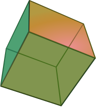
Cube (3-cube)	Tesseract (4-cube)

In geometry, a hypercube is an n-dimensional analogue of a square (n = 2) and a cube (n = 3). It is a closed, compact, convex figure whose 1-skeleton consists of groups of opposite parallel line segments aligned in each of the space's dimensions, perpendicular to each other and of the same length. A unit hypercube's longest diagonal in n dimensions is equal to ${\displaystyle {\sqrt {n}}}$.

An n-dimensional hypercube is more commonly referred to as an n-cube or sometimes as an n-dimensional cube. The term measure polytope (originally from Elte, 1912)^[1] is also used, notably in the work of H. S. M. Coxeter who also labels the hypercubes the γn polytopes.^[2]

The hypercube is the special case of a hyperrectangle (also called an n-orthotope).

A unit hypercube is a hypercube whose side has length one unit. Often, the hypercube whose corners (or vertices) are the 2ⁿ points in Rⁿ with each coordinate equal to 0 or 1 is called the unit hypercube.

Construction[]

A diagram showing how to create a tesseract from a point.

An animation showing how to create a tesseract from a point.

A hypercube can be defined by increasing the numbers of dimensions of a shape:

0 – A point is a hypercube of dimension zero.

1 – If one moves this point one unit length, it will sweep out a line segment, which is a unit hypercube of dimension one.

2 – If one moves this line segment its length in a perpendicular direction from itself; it sweeps out a 2-dimensional square.

3 – If one moves the square one unit length in the direction perpendicular to the plane it lies on, it will generate a 3-dimensional cube.

4 – If one moves the cube one unit length into the fourth dimension, it generates a 4-dimensional unit hypercube (a unit tesseract).

This can be generalized to any number of dimensions. This process of sweeping out volumes can be formalized mathematically as a Minkowski sum: the d-dimensional hypercube is the Minkowski sum of d mutually perpendicular unit-length line segments, and is therefore an example of a zonotope.

The 1-skeleton of a hypercube is a hypercube graph.

Vertex coordinates[]

A unit hypercube of dimension ${\displaystyle n}$ is the convex hull of all the points whose ${\displaystyle n}$ Cartesian coordinates are each equal to either ${\displaystyle 0}$ or ${\displaystyle 1}$. This hypercube is also the cartesian product ${\displaystyle [0,1]^{n}}$ of ${\displaystyle n}$ copies of the unit interval ${\displaystyle [0,1]}$. Another unit hypercube, centered at the origin of the ambient space, can be obtained from this one by a translation. It is the convex hull of the points whose vectors of Cartesian coordinates are

${\displaystyle \left(\pm {\frac {1}{2}},\pm {\frac {1}{2}},\cdots ,\pm {\frac {1}{2}}\right)\!\!.}$

Here the symbol ${\displaystyle \pm }$ means that each coordinate is either equal to ${\displaystyle 1/2}$ or to ${\displaystyle -1/2}$. This unit hypercube is also the cartesian product ${\displaystyle [-1/2,1/2]^{n}}$. Any unit hypercube has an edge length of ${\displaystyle 1}$ and an ${\displaystyle n}$-dimensional volume of ${\displaystyle 1}$.

The ${\displaystyle n}$-dimensional hypercube obtained as the convex hull of the points with coordinates ${\displaystyle (\pm 1,\pm 1,\cdots ,\pm 1)}$ or, equivalently as the Cartesian product ${\displaystyle [-1,1]^{n}}$ is also often considered due to the simpler form of its vertex coordinates. Its edge length is ${\displaystyle 2}$, and its ${\displaystyle n}$-dimensional volume is ${\displaystyle 2^{n}}$.

Faces[]

Every hypercube admits, as its faces, hypercubes of a lower dimension contained in its boundary. A hypercube of dimension ${\displaystyle n}$ admits ${\displaystyle 2n}$ facets, or faces of dimension ${\displaystyle n-1}$: a (${\displaystyle 1}$-dimensional) line segment has ${\displaystyle 2}$ endpoints; a (${\displaystyle 2}$-dimensional) square has ${\displaystyle 4}$ sides or edges; a ${\displaystyle 3}$-dimensional cube has ${\displaystyle 6}$ square faces; a (${\displaystyle 4}$-dimensional) tesseract has ${\displaystyle 8}$ three-dimensional cube as its facets. The number of vertices of a hypercube of dimension ${\displaystyle n}$ is ${\displaystyle 2^{n}}$ (a usual, ${\displaystyle 3}$-dimensional cube has ${\displaystyle 2^{3}=8}$ vertices, for instance).

The number of the ${\displaystyle m}$-dimensional hypercubes (just referred to as ${\displaystyle m}$-cubes from here on) contained in the boundary of an ${\displaystyle n}$-cube is

${\displaystyle E_{m,n}=2^{n-m}{n \choose m}}$,^[3]     where ${\displaystyle {n \choose m}={\frac {n!}{m!\,(n-m)!}}}$ and ${\displaystyle n!}$ denotes the factorial of ${\displaystyle n}$.

For example, the boundary of a ${\displaystyle 4}$-cube (${\displaystyle n=4}$) contains ${\displaystyle 8}$ cubes (${\displaystyle 3}$-cubes), ${\displaystyle 24}$ squares (${\displaystyle 2}$-cubes), ${\displaystyle 32}$ line segments (${\displaystyle 1}$-cubes) and ${\displaystyle 16}$ vertices (${\displaystyle 0}$-cubes). This identity can be proven by a simple combinatorial argument: for each of the ${\displaystyle 2^{n}}$ vertices of the hypercube, there are ${\displaystyle {\tbinom {n}{m}}}$ ways to choose a collection of ${\displaystyle m}$ edges incident to that vertex. Each of these collections defines one of the ${\displaystyle m}$-dimensional faces incident to the considered vertex. Doing this for all the vertices of the hypercube, each of the ${\displaystyle m}$-dimensional faces of the hypercube is counted ${\displaystyle 2^{m}}$ times since it has that many vertices, and we need to divide ${\displaystyle 2^{n}{\tbinom {n}{m}}}$ by this number.

The number of facets of the hypercube can be used to compute the ${\displaystyle (n-1)}$-dimensional volume of its boundary: that volume is ${\displaystyle 2n}$ times the volume of a ${\displaystyle (n-1)}$-dimensional hypercube; that is, ${\displaystyle 2ns^{n-1}}$ where ${\displaystyle s}$ is the length of the edges of the hypercube.

These numbers can also be generated by the linear recurrence relation

${\displaystyle E_{m,n}=2E_{m,n-1}+E_{m-1,n-1}\!}$,     with ${\displaystyle E_{0,0}=1}$, and ${\displaystyle E_{m,n}=0}$ when ${\displaystyle n<m}$, ${\displaystyle n<0}$, or ${\displaystyle m<0}$.

For example, extending a square via its 4 vertices adds one extra line segment (edge) per vertex. Adding the opposite square to form a cube provides ${\displaystyle E_{1,3}=12}$ line segments.

Number ${\displaystyle E_{m,n}}$ of ${\displaystyle m}$-dimensional faces of a ${\displaystyle n}$-dimensional hypercube (sequence A038207 in the OEIS)

			m	0	1	2	3	4	5	6	7	8	9	10
n	n-cube	Names	Schläfli Coxeter	Vertex 0-face	Edge 1-face	Face 2-face	Cell 3-face	4-face	5-face	6-face	7-face	8-face	9-face	10-face
0	0-cube	Point Monon	( )	1
1	1-cube	Line segment Dion[4]	{}	2	1
2	2-cube	Square Tetragon	{4}	4	4	1
3	3-cube	Cube Hexahedron	{4,3}	8	12	6	1
4	4-cube	Tesseract Octachoron	{4,3,3}	16	32	24	8	1
5	5-cube	Penteract Deca-5-tope	{4,3,3,3}	32	80	80	40	10	1
6	6-cube	Hexeract Dodeca-6-tope	{4,3,3,3,3}	64	192	240	160	60	12	1
7	7-cube	Hepteract Tetradeca-7-tope	{4,3,3,3,3,3}	128	448	672	560	280	84	14	1
8	8-cube	Octeract Hexadeca-8-tope	{4,3,3,3,3,3,3}	256	1024	1792	1792	1120	448	112	16	1
9	9-cube	Enneract Octadeca-9-tope	{4,3,3,3,3,3,3,3}	512	2304	4608	5376	4032	2016	672	144	18	1
10	10-cube	Dekeract Icosa-10-tope	{4,3,3,3,3,3,3,3,3}	1024	5120	11520	15360	13440	8064	3360	960	180	20	1

Graphs[]

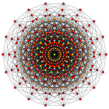
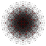
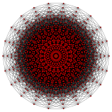
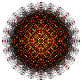
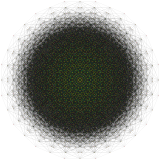
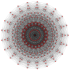
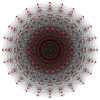
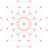
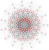
An n-cube can be projected inside a regular 2n-gonal polygon by a skew orthogonal projection, shown here from the line segment to the 15-cube.

Petrie polygon Orthographic projections

Point	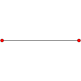Line segment	Square	Cube	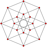Tesseract
5-cube	6-cube	7-cube	8-cube
9-cube	10-cube	11-cube	12-cube
13-cube	14-cube	15-cube	16-cube

Projection of a rotating tesseract.

Related families of polytopes[]

The hypercubes are one of the few families of regular polytopes that are represented in any number of dimensions.

The hypercube (offset) family is one of three regular polytope families, labeled by Coxeter as γ_n. The other two are the hypercube dual family, the cross-polytopes, labeled as β_n, and the simplices, labeled as α_n. A fourth family, the infinite tessellations of hypercubes, he labeled as δ_n.

Another related family of semiregular and uniform polytopes is the demihypercubes, which are constructed from hypercubes with alternate vertices deleted and simplex facets added in the gaps, labeled as hγ_n.

n-cubes can be combined with their duals (the cross-polytopes) to form compound polytopes:

• In two dimensions, we obtain the octagrammic star figure {8/2},
• In three dimensions we obtain the compound of cube and octahedron,
• In four dimensions we obtain the compound of tesseract and 16-cell.

Relation to (n−1)-simplices[]

The graph of the n-hypercube's edges is isomorphic to the Hasse diagram of the (n−1)-simplex's face lattice. This can be seen by orienting the n-hypercube so that two opposite vertices lie vertically, corresponding to the (n−1)-simplex itself and the null polytope, respectively. Each vertex connected to the top vertex then uniquely maps to one of the (n−1)-simplex's facets (n−2 faces), and each vertex connected to those vertices maps to one of the simplex's n−3 faces, and so forth, and the vertices connected to the bottom vertex map to the simplex's vertices.

This relation may be used to generate the face lattice of an (n−1)-simplex efficiently, since face lattice enumeration algorithms applicable to general polytopes are more computationally expensive.

Generalized hypercubes[]

Regular complex polytopes can be defined in complex Hilbert space called generalized hypercubes, γ^p
_n = _p{4}₂{3}...₂{3}₂, or ... Real solutions exist with p = 2, i.e. γ²
_n = γ_n = ₂{4}₂{3}...₂{3}₂ = {4,3,..,3}. For p > 2, they exist in ${\displaystyle \mathbb {C} ^{n}}$. The facets are generalized (n−1)-cube and the vertex figure are regular simplexes.

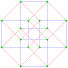
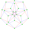
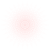
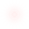
The regular polygon perimeter seen in these orthogonal projections is called a petrie polygon. The generalized squares (n = 2) are shown with edges outlined as red and blue alternating color p-edges, while the higher n-cubes are drawn with black outlined p-edges.

The number of m-face elements in a p-generalized n-cube are: ${\displaystyle p^{n-m}{n \choose m}}$. This is pⁿ vertices and pn facets.^[5]

Generalized hypercubes

	p=2		p=3	p=4	p=5	p=6	p=7	p=8
${\displaystyle \mathbb {R} ^{2}}$	γ2 2 = {4} = 4 vertices	${\displaystyle \mathbb {C} ^{2}}$	γ3 2 = 9 vertices	γ4 2 = 16 vertices	γ5 2 = 25 vertices	γ6 2 = 36 vertices	γ7 2 = 49 vertices	γ8 2 = 64 vertices
${\displaystyle \mathbb {R} ^{3}}$	γ2 3 = {4,3} = 8 vertices	${\displaystyle \mathbb {C} ^{3}}$	γ3 3 = 27 vertices	γ4 3 = 64 vertices	γ5 3 = 125 vertices	γ6 3 = 216 vertices	γ7 3 = 343 vertices	γ8 3 = 512 vertices
${\displaystyle \mathbb {R} ^{4}}$	γ2 4 = {4,3,3} = 16 vertices	${\displaystyle \mathbb {C} ^{4}}$	γ3 4 = 81 vertices	γ4 4 = 256 vertices	γ5 4 = 625 vertices	γ6 4 = 1296 vertices	γ7 4 = 2401 vertices	γ8 4 = 4096 vertices
${\displaystyle \mathbb {R} ^{5}}$	γ2 5 = {4,3,3,3} = 32 vertices	${\displaystyle \mathbb {C} ^{5}}$	γ3 5 = 243 vertices	γ4 5 = 1024 vertices	γ5 5 = 3125 vertices	γ6 5 = 7776 vertices	γ7 5 = 16,807 vertices	γ8 5 = 32,768 vertices
${\displaystyle \mathbb {R} ^{6}}$	γ2 6 = {4,3,3,3,3} = 64 vertices	${\displaystyle \mathbb {C} ^{6}}$	γ3 6 = 729 vertices	γ4 6 = 4096 vertices	γ5 6 = 15,625 vertices	γ6 6 = 46,656 vertices	γ7 6 = 117,649 vertices	γ8 6 = 262,144 vertices
${\displaystyle \mathbb {R} ^{7}}$	γ2 7 = {4,3,3,3,3,3} = 128 vertices	${\displaystyle \mathbb {C} ^{7}}$	γ3 7 = 2187 vertices	γ4 7 = 16,384 vertices	γ5 7 = 78,125 vertices	γ6 7 = 279,936 vertices	γ7 7 = 823,543 vertices	γ8 7 = 2,097,152 vertices
${\displaystyle \mathbb {R} ^{8}}$	γ2 8 = {4,3,3,3,3,3,3} = 256 vertices	${\displaystyle \mathbb {C} ^{8}}$	γ3 8 = 6561 vertices	γ4 8 = 65,536 vertices	γ5 8 = 390,625 vertices	γ6 8 = 1,679,616 vertices	γ7 8 = 5,764,801 vertices	γ8 8 = 16,777,216 vertices

See also[]

• Hypercube interconnection network of computer architecture
• Hyperoctahedral group, the symmetry group of the hypercube
• Hypersphere
• Simplex
• Parallelotope
• Crucifixion (Corpus Hypercubus) (famous artwork)

Notes[]

References[]

• Bowen, J. P. (April 1982). "Hypercube". Practical Computing. 5 (4): 97–99. Archived from the original on 2008-06-30. Retrieved June 30, 2008.
• Coxeter, H. S. M. (1973). Regular Polytopes (3rd ed.). §7.2. see illustration Fig. 7-2C: Dover. pp. 122-123. ISBN 0-486-61480-8.CS1 maint: location (link) p. 296, Table I (iii): Regular Polytopes, three regular polytopes in n dimensions (n ≥ 5)
• Hill, Frederick J.; Gerald R. Peterson (1974). Introduction to Switching Theory and Logical Design: Second Edition. New York: John Wiley & Sons. ISBN 0-471-39882-9. Cf Chapter 7.1 "Cubical Representation of Boolean Functions" wherein the notion of "hypercube" is introduced as a means of demonstrating a distance-1 code (Gray code) as the vertices of a hypercube, and then the hypercube with its vertices so labelled is squashed into two dimensions to form either a Veitch diagram or Karnaugh map.

External links[]

Wikimedia Commons has media related to Hypercubes.

• Weisstein, Eric W. "Hypercube". MathWorld.
• Weisstein, Eric W. "Hypercube graphs". MathWorld.
• www.4d-screen.de (Rotation of 4D – 7D-Cube)
• Rotating a Hypercube by Enrique Zeleny, Wolfram Demonstrations Project.
• Stereoscopic Animated Hypercube
• Rudy Rucker and Farideh Dormishian's Hypercube Downloads
• A001787    Number of edges in an n-dimensional hypercube. at OEIS