Restricted Boltzmann machine

Part of a series on
Machine learning and data mining
show Problems Classification Clustering Regression Anomaly detection Data Cleaning AutoML Association rules Reinforcement learning Structured prediction Feature engineering Feature learning Online learning Semi-supervised learning Unsupervised learning Learning to rank Grammar induction
show Supervised learning (classification • regression) Decision trees Ensembles Bagging Boosting Random forest k-NN Linear regression Naive Bayes Artificial neural networks Logistic regression Perceptron Relevance vector machine (RVM) Support vector machine (SVM)
show Clustering BIRCH CURE Hierarchical k-means Expectation–maximization (EM) DBSCAN OPTICS Mean shift
show Dimensionality reduction Factor analysis CCA ICA LDA NMF PCA PGD t-SNE
show Structured prediction Graphical models Bayes net Conditional random field Hidden Markov
show Anomaly detection k-NN Local outlier factor
hide Artificial neural network Autoencoder Cognitive computing Deep learning DeepDream Multilayer perceptron RNN LSTM GRU ESN Restricted Boltzmann machine GAN SOM Convolutional neural network U-Net Transformer Spiking neural network Memtransistor Electrochemical RAM (ECRAM)
show Reinforcement learning Q-learning SARSA Temporal difference (TD)
show Theory Bias–variance tradeoff Computational learning theory Empirical risk minimization Occam learning PAC learning Statistical learning VC theory
show Machine-learning venues NeurIPS ICML ML JMLR ArXiv:cs.LG
show Related articles Glossary of artificial intelligence List of datasets for machine-learning research Outline of machine learning
v t

Diagram of a restricted Boltzmann machine with three visible units and four hidden units (no bias units).

A restricted Boltzmann machine (RBM) is a generative stochastic artificial neural network that can learn a probability distribution over its set of inputs.

RBMs were initially invented under the name Harmonium by Paul Smolensky in 1986,^[1] and rose to prominence after Geoffrey Hinton and collaborators invented fast learning algorithms for them in the mid-2000. RBMs have found applications in dimensionality reduction,^[2] classification,^[3] collaborative filtering,^[4] feature learning,^[5] topic modelling^[6] and even many body quantum mechanics.^[7][8] They can be trained in either supervised or unsupervised ways, depending on the task.

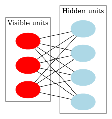
As their name implies, RBMs are a variant of Boltzmann machines, with the restriction that their neurons must form a bipartite graph: a pair of nodes from each of the two groups of units (commonly referred to as the "visible" and "hidden" units respectively) may have a symmetric connection between them; and there are no connections between nodes within a group. By contrast, "unrestricted" Boltzmann machines may have connections between hidden units. This restriction allows for more efficient training algorithms than are available for the general class of Boltzmann machines, in particular the gradient-based contrastive divergence algorithm.^[9]

Restricted Boltzmann machines can also be used in deep learning networks. In particular, deep belief networks can be formed by "stacking" RBMs and optionally fine-tuning the resulting deep network with gradient descent and backpropagation.^[10]

Structure[]

The standard type of RBM has binary-valued (Boolean) hidden and visible units, and consists of a matrix of weights ${\displaystyle W}$ of size ${\displaystyle m\times n}$. Each weight element ${\displaystyle (w_{i,j})}$ of the matrix is associated with the connection between the visible (input) unit ${\displaystyle v_{i}}$ and the hidden unit ${\displaystyle h_{j}}$. In addition, there are bias weights (offsets) ${\displaystyle a_{i}}$ for ${\displaystyle v_{i}}$ and ${\displaystyle b_{j}}$ for ${\displaystyle h_{j}}$. Given the weights and biases, the energy of a configuration (pair of boolean vectors) (v,h) is defined as

${\displaystyle E(v,h)=-\sum _{i}a_{i}v_{i}-\sum _{j}b_{j}h_{j}-\sum _{i}\sum _{j}v_{i}w_{i,j}h_{j}}$

or, in matrix notation,

${\displaystyle E(v,h)=-a^{\mathrm {T} }v-b^{\mathrm {T} }h-v^{\mathrm {T} }Wh.}$

This energy function is analogous to that of a Hopfield network. As with general Boltzmann machines, the joint probability distribution for the visible and hidden vectors is defined in terms of the energy function as follows,^[11]

${\displaystyle P(v,h)={\frac {1}{Z}}e^{-E(v,h)}}$

where ${\displaystyle Z}$ is a partition function defined as the sum of ${\displaystyle e^{-E(v,h)}}$ over all possible configurations, which can be interpreted as a normalizing constant to ensure that the probabilities sum to 1. The marginal probability of a visible vector is the sum of ${\displaystyle P(v,h)}$ over all possible hidden layer configurations,^[11]

${\displaystyle P(v)={\frac {1}{Z}}\sum _{\{h\}}e^{-E(v,h)}}$,

and vice versa. Since the underlying graph structure of the RBM is bipartite (meaning there is no intra-layer connections), the hidden unit activations are mutually independent given the visible unit activations. Conversely, the visible unit activations are mutually independent given the hidden unit activations.^[9] That is, for m visible units and n hidden units, the conditional probability of a configuration of the visible units v, given a configuration of the hidden units h, is

${\displaystyle P(v|h)=\prod _{i=1}^{m}P(v_{i}|h)}$.

Conversely, the conditional probability of h given v is

${\displaystyle P(h|v)=\prod _{j=1}^{n}P(h_{j}|v)}$.

The individual activation probabilities are given by

${\displaystyle P(h_{j}=1|v)=\sigma \left(b_{j}+\sum _{i=1}^{m}w_{i,j}v_{i}\right)}$ and ${\displaystyle \,P(v_{i}=1|h)=\sigma \left(a_{i}+\sum _{j=1}^{n}w_{i,j}h_{j}\right)}$

where ${\displaystyle \sigma }$ denotes the logistic sigmoid.

The visible units of Restricted Boltzmann Machine can be multinomial, although the hidden units are Bernoulli.^{[clarification needed]} In this case, the logistic function for visible units is replaced by the softmax function

${\displaystyle P(v_{i}^{k}=1|h)={\frac {\exp(a_{i}^{k}+\Sigma _{j}W_{ij}^{k}h_{j})}{\Sigma _{k'=1}^{K}\exp(a_{i}^{k'}+\Sigma _{j}W_{ij}^{k'}h_{j})}}}$

where K is the number of discrete values that the visible values have. They are applied in topic modeling,^[6] and recommender systems.^[4]

Relation to other models[]

Restricted Boltzmann machines are a special case of Boltzmann machines and Markov random fields.^[12][13] Their graphical model corresponds to that of factor analysis.^[14]

Training algorithm[]

Restricted Boltzmann machines are trained to maximize the product of probabilities assigned to some training set ${\displaystyle V}$ (a matrix, each row of which is treated as a visible vector ${\displaystyle v}$),

${\displaystyle \arg \max _{W}\prod _{v\in V}P(v)}$

or equivalently, to maximize the expected log probability of a training sample ${\displaystyle v}$ selected randomly from ${\displaystyle V}$:^[12][13]

${\displaystyle \arg \max _{W}\mathbb {E} \left[\log P(v)\right]}$

The algorithm most often used to train RBMs, that is, to optimize the weight vector ${\displaystyle W}$, is the contrastive divergence (CD) algorithm due to Hinton, originally developed to train PoE (product of experts) models.^[15][16] The algorithm performs Gibbs sampling and is used inside a gradient descent procedure (similar to the way backpropagation is used inside such a procedure when training feedforward neural nets) to compute weight update.

The basic, single-step contrastive divergence (CD-1) procedure for a single sample can be summarized as follows:

1. Take a training sample v, compute the probabilities of the hidden units and sample a hidden activation vector h from this probability distribution.
2. Compute the outer product of v and h and call this the positive gradient.
3. From h, sample a reconstruction v' of the visible units, then resample the hidden activations h' from this. (Gibbs sampling step)
4. Compute the outer product of v' and h' and call this the negative gradient.
5. Let the update to the weight matrix ${\displaystyle W}$ be the positive gradient minus the negative gradient, times some learning rate: ${\displaystyle \Delta W=\epsilon (vh^{\mathsf {T}}-v'h'^{\mathsf {T}})}$.
6. Update the biases a and b analogously: ${\displaystyle \Delta a=\epsilon (v-v')}$, ${\displaystyle \Delta b=\epsilon (h-h')}$.

A Practical Guide to Training RBMs written by Hinton can be found on his homepage.^[11]

Literature[]

• Fischer, Asja; Igel, Christian (2012), "An Introduction to Restricted Boltzmann Machines", Progress in Pattern Recognition, Image Analysis, Computer Vision, and Applications, Berlin, Heidelberg: Springer Berlin Heidelberg, pp. 14–36, retrieved 2021-09-19

See also[]

• Autoencoder
• Helmholtz machine

References[]

External links[]

• Introduction to Restricted Boltzmann Machines. Edwin Chen's blog, July 18, 2011.
• "A Beginner's Guide to Restricted Boltzmann Machines". Archived from the original on February 11, 2017. Retrieved November 15, 2018.CS1 maint: bot: original URL status unknown (link). Deeplearning4j Documentation
• "Understanding RBMs". Archived from the original on September 20, 2016. Retrieved December 29, 2014.. Deeplearning4j Documentation
• Python implementation of Bernoulli RBM and tutorial
• SimpleRBM is a very small RBM code (24kB) useful for you to learn about how RBMs learn and work.