Singular value decomposition

Illustration of the singular value decomposition UΣV^⁎ of a real 2×2 matrix M.

• Top: The action of M, indicated by its effect on the unit disc D and the two canonical unit vectors e₁ and e₂.
• Left: The action of V^⁎, a rotation, on D, e₁, and e₂.
• Bottom: The action of Σ, a scaling by the singular values σ₁ horizontally and σ₂ vertically.
• Right: The action of U, another rotation.

In linear algebra, the singular value decomposition (SVD) is a factorization of a real or complex matrix. It generalizes the eigendecomposition of a square normal matrix with an orthonormal eigenbasis to any ${\displaystyle m\times n}$ matrix. It is related to the polar decomposition.

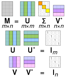
Specifically, the singular value decomposition of an ${\displaystyle m\times n}$ complex matrix M is a factorization of the form ${\displaystyle \mathbf {U\Sigma V^{*}} }$, where U is an ${\displaystyle m\times m}$ complex unitary matrix, ${\displaystyle \mathbf {\Sigma } }$ is an ${\displaystyle m\times n}$ rectangular diagonal matrix with non-negative real numbers on the diagonal, and V is an ${\displaystyle n\times n}$ complex unitary matrix. If M is real, U and V can also be guaranteed to be real orthogonal matrices. In such contexts, the SVD is often denoted ${\displaystyle \mathbf {U\Sigma V^{T}} }$.

The diagonal entries ${\displaystyle \sigma _{i}=\Sigma _{ii}}$ of ${\displaystyle \mathbf {\Sigma } }$ are known as the singular values of M. The number of non-zero singular values is equal to the rank of M. The columns of U and the columns of V are called the left-singular vectors and right-singular vectors of M, respectively.

The SVD is not unique. It is always possible to choose the decomposition so that the singular values ${\displaystyle \Sigma _{ii}}$are in descending order. In this case, ${\displaystyle \mathbf {\Sigma } }$ (but not always U and V) is uniquely determined by M.

The term sometimes refers to the compact SVD, a similar decomposition ${\displaystyle \mathbf {M} =\mathbf {U\Sigma V^{*}} }$ in which ${\displaystyle \mathbf {\Sigma } }$ is square diagonal of size ${\displaystyle r\times r}$, where ${\displaystyle r\leq \min\{m,n\}}$ is the rank of M, and has only the non-zero singular values. In this variant, U is an ${\displaystyle m\times r}$ semi-unitary matrix and ${\displaystyle \mathbf {V} }$ is an ${\displaystyle n\times r}$ semi-unitary matrix, such that ${\displaystyle \mathbf {U^{*}U} =\mathbf {V^{*}V} =\mathbf {I} _{r}}$.

Mathematical applications of the SVD include computing the pseudoinverse, matrix approximation, and determining the rank, range, and null space of a matrix. The SVD is also extremely useful in all areas of science, engineering, and statistics, such as signal processing, least squares fitting of data, and process control.

Intuitive interpretations[]

Animated illustration of the SVD of a 2D, real shearing matrix M. First, we see the unit disc in blue together with the two canonical unit vectors. We then see the actions of M, which distorts the disk to an ellipse. The SVD decomposes M into three simple transformations: an initial rotation V^⁎, a scaling ${\displaystyle \mathbf {\Sigma } }$ along the coordinate axes, and a final rotation U. The lengths σ₁ and σ₂ of the semi-axes of the ellipse are the singular values of M, namely Σ_1,1 and Σ_2,2.

Visualisation of the matrix multiplications in singular value decomposition

Rotation, coordinate scaling, and reflection[]

In the special case when M is an m × m real square matrix, the matrices U and V^⁎ can be chosen to be real m × m matrices too. In that case, "unitary" is the same as "orthogonal". Then, interpreting both unitary matrices as well as the diagonal matrix, summarized here as A, as a linear transformation x ↦ Ax of the space R^m, the matrices U and V^⁎ represent rotations or reflection of the space, while ${\displaystyle \mathbf {\Sigma } }$ represents the scaling of each coordinate x_i by the factor σ_i. Thus the SVD decomposition breaks down any invertible linear transformation of R^m into a composition of three geometrical transformations: a rotation or reflection (V^⁎), followed by a coordinate-by-coordinate scaling (${\displaystyle \mathbf {\Sigma } }$), followed by another rotation or reflection (U).

In particular, if M has a positive determinant, then U and V^⁎ can be chosen to be both reflections, or both rotations. If the determinant is negative, exactly one of them will have to be a reflection. If the determinant is zero, each can be independently chosen to be of either type.

If the matrix M is real but not square, namely m×n with m ≠ n, it can be interpreted as a linear transformation from Rⁿ to R^m. Then U and V^⁎ can be chosen to be rotations of R^m and Rⁿ, respectively; and ${\displaystyle \mathbf {\Sigma } }$, besides scaling the first ${\displaystyle \min\{m,n\}}$ coordinates, also extends the vector with zeros, i.e. removes trailing coordinates, so as to turn Rⁿ into R^m.

Singular values as semiaxes of an ellipse or ellipsoid[]

As shown in the figure, the singular values can be interpreted as the magnitude of the semiaxes of an ellipse in 2D. This concept can be generalized to n-dimensional Euclidean space, with the singular values of any n × n square matrix being viewed as the magnitude of the semiaxis of an n-dimensional ellipsoid. Similarly, the singular values of any m × n matrix can be viewed as the magnitude of the semiaxis of an n-dimensional ellipsoid in m-dimensional space, for example as an ellipse in a (tilted) 2D plane in a 3D space. Singular values encode magnitude of the semiaxis, while singular vectors encode direction. See below for further details.

The columns of U and V are orthonormal bases[]

Since U and V^⁎ are unitary, the columns of each of them form a set of orthonormal vectors, which can be regarded as basis vectors. The matrix M maps the basis vector V_i to the stretched unit vector σ_i U_i. By the definition of a unitary matrix, the same is true for their conjugate transposes U^⁎ and V, except the geometric interpretation of the singular values as stretches is lost. In short, the columns of U, U^⁎, V, and V^⁎ are orthonormal bases. When the ${\displaystyle \mathbf {M} }$ is a normal matrix, U and V are both equal to the unitary matrix used to diagonalize ${\displaystyle \mathbf {M} }$. However, when ${\displaystyle \mathbf {M} }$ is not normal but still diagonalizable, its eigendecomposition and singular value decomposition are distinct.

Geometric meaning[]

Because U and V are unitary, we know that the columns U₁, ..., U_m of U yield an orthonormal basis of K^m and the columns V₁, ..., V_n of V yield an orthonormal basis of Kⁿ (with respect to the standard scalar products on these spaces).

The linear transformation

${\displaystyle {\begin{cases}T:K^{n}\to K^{m}\\x\mapsto \mathbf {M} x\end{cases}}}$

has a particularly simple description with respect to these orthonormal bases: we have

${\displaystyle T(\mathbf {V} _{i})=\sigma _{i}\mathbf {U} _{i},\qquad i=1,\ldots ,\min(m,n),}$

where σ_i is the i-th diagonal entry of ${\displaystyle \mathbf {\Sigma } }$, and T(V_i) = 0 for i > min(m,n).

The geometric content of the SVD theorem can thus be summarized as follows: for every linear map T : Kⁿ → K^m one can find orthonormal bases of Kⁿ and K^m such that T maps the i-th basis vector of Kⁿ to a non-negative multiple of the i-th basis vector of K^m, and sends the left-over basis vectors to zero. With respect to these bases, the map T is therefore represented by a diagonal matrix with non-negative real diagonal entries.

To get a more visual flavor of singular values and SVD factorization – at least when working on real vector spaces – consider the sphere S of radius one in Rⁿ. The linear map T maps this sphere onto an ellipsoid in R^m. Non-zero singular values are simply the lengths of the semi-axes of this ellipsoid. Especially when n = m, and all the singular values are distinct and non-zero, the SVD of the linear map T can be easily analyzed as a succession of three consecutive moves: consider the ellipsoid T(S) and specifically its axes; then consider the directions in Rⁿ sent by T onto these axes. These directions happen to be mutually orthogonal. Apply first an isometry V^⁎ sending these directions to the coordinate axes of Rⁿ. On a second move, apply an endomorphism D diagonalized along the coordinate axes and stretching or shrinking in each direction, using the semi-axes lengths of T(S) as stretching coefficients. The composition D ∘ V^⁎ then sends the unit-sphere onto an ellipsoid isometric to T(S). To define the third and last move U, apply an isometry to this ellipsoid so as to carry it over T(S)^{[clarification needed]}. As can be easily checked, the composition U ∘ D ∘ V^⁎ coincides with T.

Example[]

Consider the 4 × 5 matrix

${\displaystyle \mathbf {M} ={\begin{bmatrix}1&0&0&0&2\\0&0&3&0&0\\0&0&0&0&0\\0&2&0&0&0\end{bmatrix}}}$

A singular value decomposition of this matrix is given by UΣV^⁎

${\displaystyle {\begin{aligned}\mathbf {U} &={\begin{bmatrix}\color {Green}0&\color {Blue}-1&\color {Cyan}0&\color {Emerald}0\\\color {Green}-1&\color {Blue}0&\color {Cyan}0&\color {Emerald}0\\\color {Green}0&\color {Blue}0&\color {Cyan}0&\color {Emerald}-1\\\color {Green}0&\color {Blue}0&\color {Cyan}-1&\color {Emerald}0\end{bmatrix}}\\[6pt]{\boldsymbol {\Sigma }}&={\begin{bmatrix}3&0&0&0&\color {Gray}{\mathit {0}}\\0&{\sqrt {5}}&0&0&\color {Gray}{\mathit {0}}\\0&0&2&0&\color {Gray}{\mathit {0}}\\0&0&0&\color {Red}\mathbf {0} &\color {Gray}{\mathit {0}}\end{bmatrix}}\\[6pt]\mathbf {V} ^{*}&={\begin{bmatrix}\color {Violet}0&\color {Violet}0&\color {Violet}-1&\color {Violet}0&\color {Violet}0\\\color {Plum}-{\sqrt {0.2}}&\color {Plum}0&\color {Plum}0&\color {Plum}0&\color {Plum}-{\sqrt {0.8}}\\\color {Magenta}0&\color {Magenta}-1&\color {Magenta}0&\color {Magenta}0&\color {Magenta}0\\\color {Orchid}0&\color {Orchid}0&\color {Orchid}0&\color {Orchid}1&\color {Orchid}0\\\color {Purple}-{\sqrt {0.8}}&\color {Purple}0&\color {Purple}0&\color {Purple}0&\color {Purple}{\sqrt {0.2}}\end{bmatrix}}\end{aligned}}}$

The scaling matrix ${\displaystyle \mathbf {\Sigma } }$ is zero outside of the diagonal (grey italics) and one diagonal element is zero (red bold). Furthermore, because the matrices U and V^⁎ are unitary, multiplying by their respective conjugate transposes yields identity matrices, as shown below. In this case, because U and V^⁎ are real valued, each is an orthogonal matrix.

${\displaystyle {\begin{aligned}\mathbf {U} \mathbf {U} ^{*}&={\begin{bmatrix}1&0&0&0\\0&1&0&0\\0&0&1&0\\0&0&0&1\end{bmatrix}}=\mathbf {I} _{4}\\[6pt]\mathbf {V} \mathbf {V} ^{*}&={\begin{bmatrix}1&0&0&0&0\\0&1&0&0&0\\0&0&1&0&0\\0&0&0&1&0\\0&0&0&0&1\end{bmatrix}}=\mathbf {I} _{5}\end{aligned}}}$

This particular singular value decomposition is not unique. Choosing ${\displaystyle \mathbf {V} }$ such that

${\displaystyle \mathbf {V} ^{*}={\begin{bmatrix}\color {Violet}0&\color {Violet}1&\color {Violet}0&\color {Violet}0&\color {Violet}0\\\color {Plum}0&\color {Plum}0&\color {Plum}1&\color {Plum}0&\color {Plum}0\\\color {Magenta}{\sqrt {0.2}}&\color {Magenta}0&\color {Magenta}0&\color {Magenta}0&\color {Magenta}{\sqrt {0.8}}\\\color {Orchid}{\sqrt {0.4}}&\color {Orchid}0&\color {Orchid}0&\color {Orchid}{\sqrt {0.5}}&\color {Orchid}-{\sqrt {0.1}}\\\color {Purple}-{\sqrt {0.4}}&\color {Purple}0&\color {Purple}0&\color {Purple}{\sqrt {0.5}}&\color {Purple}{\sqrt {0.1}}\end{bmatrix}}}$

is also a valid singular value decomposition.

SVD and spectral decomposition[]

Singular values, singular vectors, and their relation to the SVD[]

A non-negative real number σ is a singular value for M if and only if there exist unit-length vectors ${\displaystyle \mathbf {u} }$ in K^m and ${\displaystyle \mathbf {v} }$ in Kⁿ such that

${\displaystyle \mathbf {Mv} =\sigma \mathbf {u} \,{\text{ and }}\mathbf {M} ^{*}\mathbf {u} =\sigma \mathbf {v} .}$

The vectors ${\displaystyle \mathbf {u} }$ and ${\displaystyle \mathbf {v} }$ are called left-singular and right-singular vectors for σ, respectively.

In any singular value decomposition

${\displaystyle \mathbf {M} =\mathbf {U} {\boldsymbol {\Sigma }}\mathbf {V} ^{*}}$

the diagonal entries of ${\displaystyle \mathbf {\Sigma } }$ are equal to the singular values of M. The first p = min(m, n) columns of U and V are, respectively, left- and right-singular vectors for the corresponding singular values. Consequently, the above theorem implies that:

• An m × n matrix M has at most p distinct singular values.
• It is always possible to find a unitary basis U for K^m with a subset of basis vectors spanning the left-singular vectors of each singular value of M.
• It is always possible to find a unitary basis V for Kⁿ with a subset of basis vectors spanning the right-singular vectors of each singular value of M.

A singular value for which we can find two left (or right) singular vectors that are linearly independent is called degenerate. If ${\displaystyle \mathbf {u} _{1}}$ and ${\displaystyle \mathbf {u} _{2}}$ are two left-singular vectors which both correspond to the singular value σ, then any normalized linear combination of the two vectors is also a left-singular vector corresponding to the singular value σ. The similar statement is true for right-singular vectors. The number of independent left and right-singular vectors coincides, and these singular vectors appear in the same columns of U and V corresponding to diagonal elements of ${\displaystyle \mathbf {\Sigma } }$ all with the same value σ.

As an exception, the left and right-singular vectors of singular value 0 comprise all unit vectors in the kernel and cokernel, respectively, of M, which by the rank–nullity theorem cannot be the same dimension if m ≠ n. Even if all singular values are nonzero, if m > n then the cokernel is nontrivial, in which case U is padded with m − n orthogonal vectors from the cokernel. Conversely, if m < n, then V is padded by n − m orthogonal vectors from the kernel. However, if the singular value of 0 exists, the extra columns of U or V already appear as left or right-singular vectors.

Non-degenerate singular values always have unique left- and right-singular vectors, up to multiplication by a unit-phase factor e^iφ (for the real case up to a sign). Consequently, if all singular values of a square matrix M are non-degenerate and non-zero, then its singular value decomposition is unique, up to multiplication of a column of U by a unit-phase factor and simultaneous multiplication of the corresponding column of V by the same unit-phase factor. In general, the SVD is unique up to arbitrary unitary transformations applied uniformly to the column vectors of both U and V spanning the subspaces of each singular value, and up to arbitrary unitary transformations on vectors of U and V spanning the kernel and cokernel, respectively, of M.

Relation to eigenvalue decomposition[]

The singular value decomposition is very general in the sense that it can be applied to any m × n matrix, whereas eigenvalue decomposition can only be applied to diagonalizable matrices. Nevertheless, the two decompositions are related.

Given an SVD of M, as described above, the following two relations hold:

${\displaystyle {\begin{aligned}\mathbf {M} ^{*}\mathbf {M} &=\mathbf {V} {\boldsymbol {\Sigma }}^{*}\mathbf {U} ^{*}\,\mathbf {U} {\boldsymbol {\Sigma }}\mathbf {V} ^{*}=\mathbf {V} ({\boldsymbol {\Sigma }}^{*}{\boldsymbol {\Sigma }})\mathbf {V} ^{*}\\\mathbf {M} \mathbf {M} ^{*}&=\mathbf {U} {\boldsymbol {\Sigma }}\mathbf {V} ^{*}\,\mathbf {V} {\boldsymbol {\Sigma }}^{*}\mathbf {U} ^{*}=\mathbf {U} ({\boldsymbol {\Sigma }}{\boldsymbol {\Sigma }}^{*})\mathbf {U} ^{*}\end{aligned}}}$

The right-hand sides of these relations describe the eigenvalue decompositions of the left-hand sides. Consequently:

• The columns of V (right-singular vectors) are eigenvectors of M^⁎M.
• The columns of U (left-singular vectors) are eigenvectors of MM^⁎.
• The non-zero elements of ${\displaystyle \mathbf {\Sigma } }$ (non-zero singular values) are the square roots of the non-zero eigenvalues of M^⁎M or MM^⁎.

In the special case that M is a normal matrix, which by definition must be square, the spectral theorem says that it can be unitarily diagonalized using a basis of eigenvectors, so that it can be written M = UDU^⁎ for a unitary matrix U and a diagonal matrix D. When M is also positive semi-definite, the decomposition M = UDU^⁎ is also a singular value decomposition. Otherwise, it can be recast as an SVD by moving the phase of each σ_i to either its corresponding V_i or U_i. The natural connection of the SVD to non-normal matrices is through the polar decomposition theorem: M = SR, where S = UΣU^⁎ is positive semidefinite and normal, and R = UV^⁎ is unitary.

Thus, except for positive semi-definite normal matrices, the eigenvalue decomposition and SVD of M, while related, differ: the eigenvalue decomposition is M = UDU⁻¹, where U is not necessarily unitary and D is not necessarily positive semi-definite, while the SVD is M = UΣV^⁎, where ${\displaystyle \mathbf {\Sigma } }$ is diagonal and positive semi-definite, and U and V are unitary matrices that are not necessarily related except through the matrix M. While only non-defective square matrices have an eigenvalue decomposition, any ${\displaystyle m\times n}$ matrix has a SVD.

Applications of the SVD[]

Pseudoinverse[]

The singular value decomposition can be used for computing the pseudoinverse of a matrix. (Various authors use different notation for the pseudoinverse; here we use ^†.) Indeed, the pseudoinverse of the matrix M with singular value decomposition M = UΣV^⁎ is

M^† = V Σ^† U^⁎

where Σ^† is the pseudoinverse of Σ, which is formed by replacing every non-zero diagonal entry by its reciprocal and transposing the resulting matrix. The pseudoinverse is one way to solve linear least squares problems.

Solving homogeneous linear equations[]

A set of homogeneous linear equations can be written as Ax = 0 for a matrix A and vector x. A typical situation is that A is known and a non-zero x is to be determined which satisfies the equation. Such an x belongs to A's null space and is sometimes called a (right) null vector of A. The vector x can be characterized as a right-singular vector corresponding to a singular value of A that is zero. This observation means that if A is a square matrix and has no vanishing singular value, the equation has no non-zero x as a solution. It also means that if there are several vanishing singular values, any linear combination of the corresponding right-singular vectors is a valid solution. Analogously to the definition of a (right) null vector, a non-zero x satisfying x^⁎A = 0, with x^⁎ denoting the conjugate transpose of x, is called a left null vector of A.

Total least squares minimization[]

A total least squares problem seeks the vector x that minimizes the 2-norm of a vector Ax under the constraint ||x|| = 1. The solution turns out to be the right-singular vector of A corresponding to the smallest singular value.

Range, null space and rank[]

Another application of the SVD is that it provides an explicit representation of the range and null space of a matrix M. The right-singular vectors corresponding to vanishing singular values of M span the null space of M and the left-singular vectors corresponding to the non-zero singular values of M span the range of M. For example, in the above example the null space is spanned by the last two rows of V^⁎ and the range is spanned by the first three columns of U.

As a consequence, the rank of M equals the number of non-zero singular values which is the same as the number of non-zero diagonal elements in ${\displaystyle \mathbf {\Sigma } }$. In numerical linear algebra the singular values can be used to determine the effective rank of a matrix, as rounding error may lead to small but non-zero singular values in a rank deficient matrix. Singular values beyond a significant gap are assumed to be numerically equivalent to zero.

Low-rank matrix approximation[]

Some practical applications need to solve the problem of approximating a matrix M with another matrix ${\displaystyle {\tilde {\mathbf {M} }}}$, said to be truncated, which has a specific rank r. In the case that the approximation is based on minimizing the Frobenius norm of the difference between M and ${\displaystyle {\tilde {\mathbf {M} }}}$ under the constraint that ${\displaystyle \operatorname {rank} \left({\tilde {\mathbf {M} }}\right)=r}$, it turns out that the solution is given by the SVD of M, namely

${\displaystyle {\tilde {\mathbf {M} }}=\mathbf {U} {\tilde {\boldsymbol {\Sigma }}}\mathbf {V} ^{*},}$

where ${\displaystyle {\tilde {\boldsymbol {\Sigma }}}}$ is the same matrix as ${\displaystyle \mathbf {\Sigma } }$ except that it contains only the r largest singular values (the other singular values are replaced by zero). This is known as the Eckart–Young theorem, as it was proved by those two authors in 1936 (although it was later found to have been known to earlier authors; see Stewart 1993).

Separable models[]

The SVD can be thought of as decomposing a matrix into a weighted, ordered sum of separable matrices. By separable, we mean that a matrix A can be written as an outer product of two vectors A = u ⊗ v, or, in coordinates, ${\displaystyle A_{ij}=u_{i}v_{j}}$. Specifically, the matrix M can be decomposed as

${\displaystyle \mathbf {M} =\sum _{i}\mathbf {A} _{i}=\sum _{i}\sigma _{i}\mathbf {U} _{i}\otimes \mathbf {V} _{i}.}$

Here U_i and V_i are the i-th columns of the corresponding SVD matrices, σ_i are the ordered singular values, and each A_i is separable. The SVD can be used to find the decomposition of an image processing filter into separable horizontal and vertical filters. Note that the number of non-zero σ_i is exactly the rank of the matrix.

Separable models often arise in biological systems, and the SVD factorization is useful to analyze such systems. For example, some visual area V1 simple cells' receptive fields can be well described^[1] by a Gabor filter in the space domain multiplied by a modulation function in the time domain. Thus, given a linear filter evaluated through, for example, reverse correlation, one can rearrange the two spatial dimensions into one dimension, thus yielding a two-dimensional filter (space, time) which can be decomposed through SVD. The first column of U in the SVD factorization is then a Gabor while the first column of V represents the time modulation (or vice versa). One may then define an index of separability

${\displaystyle \alpha ={\frac {\sigma _{1}^{2}}{\sum _{i}\sigma _{i}^{2}}},}$

which is the fraction of the power in the matrix M which is accounted for by the first separable matrix in the decomposition.^[2]

Nearest orthogonal matrix[]

It is possible to use the SVD of a square matrix A to determine the orthogonal matrix O closest to A. The closeness of fit is measured by the Frobenius norm of O − A. The solution is the product UV^⁎.^[3] This intuitively makes sense because an orthogonal matrix would have the decomposition UIV^⁎ where I is the identity matrix, so that if A = UΣV^⁎ then the product A = UV^⁎ amounts to replacing the singular values with ones. Equivalently, the solution is the unitary matrix R = UV^⁎ of the Polar Decomposition M = RP = P'R in either order of stretch and rotation, as described above.

A similar problem, with interesting applications in shape analysis, is the orthogonal Procrustes problem, which consists of finding an orthogonal matrix O which most closely maps A to B. Specifically,

${\displaystyle \mathbf {O} ={\underset {\Omega }{\operatorname {argmin} }}\|\mathbf {A} {\boldsymbol {\Omega }}-\mathbf {B} \|_{F}\quad {\text{subject to}}\quad {\boldsymbol {\Omega }}^{\textsf {T}}{\boldsymbol {\Omega }}=\mathbf {I} ,}$

where ${\displaystyle \|\cdot \|_{F}}$ denotes the Frobenius norm.

This problem is equivalent to finding the nearest orthogonal matrix to a given matrix M = A^TB.

The Kabsch algorithm[]

The Kabsch algorithm (called Wahba's problem in other fields) uses SVD to compute the optimal rotation (with respect to least-squares minimization) that will align a set of points with a corresponding set of points. It is used, among other applications, to compare the structures of molecules.

Signal processing[]

The SVD and pseudoinverse have been successfully applied to signal processing,^[4] image processing^{[citation needed]} and big data (e.g., in genomic signal processing).^[5][6][7][8]

Other examples[]

The SVD is also applied extensively to the study of linear inverse problems and is useful in the analysis of regularization methods such as that of Tikhonov. It is widely used in statistics, where it is related to principal component analysis and to Correspondence analysis, and in signal processing and pattern recognition. It is also used in output-only modal analysis, where the non-scaled mode shapes can be determined from the singular vectors. Yet another usage is latent semantic indexing in natural-language text processing.

In general numerical computation involving linear or linearized systems, there is a universal constant that characterizes the regularity or singularity of a problem, which is the system's "condition number" ${\displaystyle \kappa :=\sigma _{\text{max}}/\sigma _{\text{min}}}$. It often controls the error rate or convergence rate of a given computational scheme on such systems.^[9][10]

The SVD also plays a crucial role in the field of quantum information, in a form often referred to as the Schmidt decomposition. Through it, states of two quantum systems are naturally decomposed, providing a necessary and sufficient condition for them to be entangled: if the rank of the ${\displaystyle \mathbf {\Sigma } }$ matrix is larger than one.

One application of SVD to rather large matrices is in numerical weather prediction, where Lanczos methods are used to estimate the most linearly quickly growing few perturbations to the central numerical weather prediction over a given initial forward time period; i.e., the singular vectors corresponding to the largest singular values of the linearized propagator for the global weather over that time interval. The output singular vectors in this case are entire weather systems. These perturbations are then run through the full nonlinear model to generate an ensemble forecast, giving a handle on some of the uncertainty that should be allowed for around the current central prediction.

SVD has also been applied to reduced order modelling. The aim of reduced order modelling is to reduce the number of degrees of freedom in a complex system which is to be modeled. SVD was coupled with radial basis functions to interpolate solutions to three-dimensional unsteady flow problems.^[11]

Interestingly, SVD has been used to improve gravitational waveform modeling by the ground-based gravitational-wave interferometer aLIGO.^[12] SVD can help to increase the accuracy and speed of waveform generation to support gravitational-waves searches and update two different waveform models.

Singular value decomposition is used in recommender systems to predict people's item ratings.^[13] Distributed algorithms have been developed for the purpose of calculating the SVD on clusters of commodity machines.^[14]

Low-rank SVD has been applied for hotspot detection from spatiotemporal data with application to disease outbreak detection.^[15] A combination of SVD and higher-order SVD also has been applied for real time event detection from complex data streams (multivariate data with space and time dimensions) in Disease surveillance.^[16]

Existence proofs[]

An eigenvalue λ of a matrix M is characterized by the algebraic relation Mu = λu. When M is Hermitian, a variational characterization is also available. Let M be a real n × n symmetric matrix. Define

${\displaystyle {\begin{cases}f:\mathbb {R} ^{n}\to \mathbb {R} \\f:\mathbf {x} \mapsto \mathbf {x} ^{\textsf {T}}\mathbf {M} \mathbf {x} \end{cases}}}$

By the extreme value theorem, this continuous function attains a maximum at some u when restricted to the unit sphere {||x|| = 1}. By the Lagrange multipliers theorem, u necessarily satisfies

${\displaystyle \nabla \mathbf {u} ^{\textsf {T}}\mathbf {M} \mathbf {u} -\lambda \cdot \nabla \mathbf {u} ^{\textsf {T}}\mathbf {u} =0}$

for some real number λ. The nabla symbol, ∇, is the del operator (differentiation with respect to x). Using the symmetry of M we obtain

${\displaystyle \nabla \mathbf {x} ^{\textsf {T}}\mathbf {M} \mathbf {x} -\lambda \cdot \nabla \mathbf {x} ^{\textsf {T}}\mathbf {x} =2(\mathbf {M} -\lambda \mathbf {I} )\mathbf {x} .}$

Therefore Mu = λu, so u is a unit length eigenvector of M. For every unit length eigenvector v of M its eigenvalue is f(v), so λ is the largest eigenvalue of M. The same calculation performed on the orthogonal complement of u gives the next largest eigenvalue and so on. The complex Hermitian case is similar; there f(x) = x* M x is a real-valued function of 2n real variables.

Singular values are similar in that they can be described algebraically or from variational principles. Although, unlike the eigenvalue case, Hermiticity, or symmetry, of M is no longer required.

This section gives these two arguments for existence of singular value decomposition.

Based on the spectral theorem[]

Let ${\displaystyle \mathbf {M} }$ be an m × n complex matrix. Since ${\displaystyle \mathbf {M} ^{*}\mathbf {M} }$ is positive semi-definite and Hermitian, by the spectral theorem, there exists an n × n unitary matrix ${\displaystyle \mathbf {V} }$ such that

${\displaystyle \mathbf {V} ^{*}\mathbf {M} ^{*}\mathbf {M} \mathbf {V} ={\bar {\mathbf {D} }}={\begin{bmatrix}\mathbf {D} &0\\0&0\end{bmatrix}},}$

where ${\displaystyle \mathbf {D} }$ is diagonal and positive definite, of dimension ${\displaystyle \ell \times \ell }$, with ${\displaystyle \ell }$ the number of non-zero eigenvalues of ${\displaystyle \mathbf {M} ^{*}\mathbf {M} }$ (which can be shown to verify ${\displaystyle \ell \leq \min(n,m)}$). Note that ${\displaystyle \mathbf {V} }$ is here by definition a matrix whose ${\displaystyle i}$-th column is the ${\displaystyle i}$-th eigenvector of ${\displaystyle \mathbf {M} ^{*}\mathbf {M} }$, corresponding to the eigenvalue ${\displaystyle {\bar {\mathbf {D} }}_{ii}}$. Moreover, the ${\displaystyle j}$-th column of ${\displaystyle \mathbf {V} }$, for ${\displaystyle j>\ell }$, is an eigenvector of ${\displaystyle \mathbf {M} ^{*}\mathbf {M} }$ with eigenvalue ${\displaystyle {\bar {\mathbf {D} }}_{jj}=0}$. This can be expressed by writing ${\displaystyle \mathbf {V} }$ as ${\displaystyle \mathbf {V} ={\begin{bmatrix}\mathbf {V} _{1}&\mathbf {V} _{2}\end{bmatrix}}}$, where the columns of ${\displaystyle \mathbf {V} _{1}}$ and ${\displaystyle \mathbf {V} _{2}}$ therefore contain the eigenvectors of ${\displaystyle \mathbf {M} ^{*}\mathbf {M} }$ corresponding to non-zero and zero eigenvalues, respectively. Using this rewriting of ${\displaystyle \mathbf {V} }$, the equation becomes:

${\displaystyle {\begin{bmatrix}\mathbf {V} _{1}^{*}\\\mathbf {V} _{2}^{*}\end{bmatrix}}\mathbf {M} ^{*}\mathbf {M} {\begin{bmatrix}\mathbf {V} _{1}&\mathbf {V} _{2}\end{bmatrix}}={\begin{bmatrix}\mathbf {V} _{1}^{*}\mathbf {M} ^{*}\mathbf {M} \mathbf {V} _{1}&\mathbf {V} _{1}^{*}\mathbf {M} ^{*}\mathbf {M} \mathbf {V} _{2}\\\mathbf {V} _{2}^{*}\mathbf {M} ^{*}\mathbf {M} \mathbf {V} _{1}&\mathbf {V} _{2}^{*}\mathbf {M} ^{*}\mathbf {M} \mathbf {V} _{2}\end{bmatrix}}={\begin{bmatrix}\mathbf {D} &0\\0&0\end{bmatrix}}.}$

This implies that

${\displaystyle \mathbf {V} _{1}^{*}\mathbf {M} ^{*}\mathbf {M} \mathbf {V} _{1}=\mathbf {D} ,\quad \mathbf {V} _{2}^{*}\mathbf {M} ^{*}\mathbf {M} \mathbf {V} _{2}=\mathbf {0} .}$

Moreover, the second equation implies ${\displaystyle \mathbf {M} \mathbf {V} _{2}=\mathbf {0} }$.^[17] Finally, the unitary-ness of ${\displaystyle \mathbf {V} }$ translates, in terms of ${\displaystyle \mathbf {V} _{1}}$ and ${\displaystyle \mathbf {V} _{2}}$, into the following conditions:

${\displaystyle {\begin{aligned}\mathbf {V} _{1}^{*}\mathbf {V} _{1}&=\mathbf {I} _{1},\\\mathbf {V} _{2}^{*}\mathbf {V} _{2}&=\mathbf {I} _{2},\\\mathbf {V} _{1}\mathbf {V} _{1}^{*}+\mathbf {V} _{2}\mathbf {V} _{2}^{*}&=\mathbf {I} _{12},\end{aligned}}}$

where the subscripts on the identity matrices are used to remark that they are of different dimensions.

Let us now define

${\displaystyle \mathbf {U} _{1}=\mathbf {M} \mathbf {V} _{1}\mathbf {D} ^{-{\frac {1}{2}}}.}$

Then,

${\displaystyle \mathbf {U} _{1}\mathbf {D} ^{\frac {1}{2}}\mathbf {V} _{1}^{*}=\mathbf {M} \mathbf {V} _{1}\mathbf {D} ^{-{\frac {1}{2}}}\mathbf {D} ^{\frac {1}{2}}\mathbf {V} _{1}^{*}=\mathbf {M} (\mathbf {I} -\mathbf {V} _{2}\mathbf {V} _{2}^{*})=\mathbf {M} -(\mathbf {M} \mathbf {V} _{2})\mathbf {V} _{2}^{*}=\mathbf {M} ,}$

since ${\displaystyle \mathbf {M} \mathbf {V} _{2}=\mathbf {0} .}$ This can be also seen as immediate consequence of the fact that ${\displaystyle \mathbf {M} \mathbf {V} _{1}\mathbf {V} _{1}^{*}=\mathbf {M} }$. Note how this is equivalent to the observation that, if ${\displaystyle \{{\boldsymbol {v}}_{i}\}_{i=1}^{\ell }}$ is the set of eigenvectors of ${\displaystyle \mathbf {M} ^{*}\mathbf {M} }$ corresponding to non-vanishing eigenvalues, then ${\displaystyle \{\mathbf {M} {\boldsymbol {v}}_{i}\}_{i=1}^{\ell }}$ is a set of orthogonal vectors, and ${\displaystyle \{\lambda ^{-1/2}\mathbf {M} {\boldsymbol {v}}_{i}\}_{i=1}^{\ell }}$ a (generally not complete) set of orthonormal vectors. This matches with the matrix formalism used above denoting with ${\displaystyle \mathbf {V} _{1}}$ the matrix whose columns are ${\displaystyle \{{\boldsymbol {v}}_{i}\}_{i=1}^{\ell }}$, with ${\displaystyle \mathbf {V} _{2}}$ the matrix whose columns are the eigenvectors of ${\displaystyle \mathbf {M} ^{*}\mathbf {M} }$ which vanishing eigenvalue, and ${\displaystyle \mathbf {U} _{1}}$ the matrix whose columns are the vectors ${\displaystyle \{\lambda ^{-1/2}\mathbf {M} {\boldsymbol {v}}_{i}\}_{i=1}^{\ell }}$.

We see that this is almost the desired result, except that ${\displaystyle \mathbf {U} _{1}}$ and ${\displaystyle \mathbf {V} _{1}}$ are in general not unitary, since they might not be square. However, we do know that the number of rows of ${\displaystyle \mathbf {U} _{1}}$ is no smaller than the number of columns, since the dimensions of ${\displaystyle \mathbf {D} }$ is no greater than ${\displaystyle m}$ and ${\displaystyle n}$. Also, since

${\displaystyle \mathbf {U} _{1}^{*}\mathbf {U} _{1}=\mathbf {D} ^{-{\frac {1}{2}}}\mathbf {V} _{1}^{*}\mathbf {M} ^{*}\mathbf {M} \mathbf {V} _{1}\mathbf {D} ^{-{\frac {1}{2}}}=\mathbf {D} ^{-{\frac {1}{2}}}\mathbf {D} \mathbf {D} ^{-{\frac {1}{2}}}=\mathbf {I_{1}} ,}$

the columns in ${\displaystyle \mathbf {U} _{1}}$ are orthonormal and can be extended to an orthonormal basis. This means that we can choose ${\displaystyle \mathbf {U} _{2}}$ such that ${\displaystyle \mathbf {U} ={\begin{bmatrix}\mathbf {U} _{1}&\mathbf {U} _{2}\end{bmatrix}}}$ is unitary.

For V₁ we already have V₂ to make it unitary. Now, define

${\displaystyle {\boldsymbol {\Sigma }}={\begin{bmatrix}{\begin{bmatrix}\mathbf {D} ^{\frac {1}{2}}&0\\0&0\end{bmatrix}}\\0\end{bmatrix}},}$

where extra zero rows are added or removed to make the number of zero rows equal the number of columns of U₂, and hence the overall dimensions of ${\displaystyle {\boldsymbol {\Sigma }}}$ equal to ${\displaystyle m\times n}$. Then

${\displaystyle {\begin{bmatrix}\mathbf {U} _{1}&\mathbf {U} _{2}\end{bmatrix}}{\begin{bmatrix}{\begin{bmatrix}\mathbf {} D^{\frac {1}{2}}&0\\0&0\end{bmatrix}}\\0\end{bmatrix}}{\begin{bmatrix}\mathbf {V} _{1}&\mathbf {V} _{2}\end{bmatrix}}^{*}={\begin{bmatrix}\mathbf {U} _{1}&\mathbf {U} _{2}\end{bmatrix}}{\begin{bmatrix}\mathbf {D} ^{\frac {1}{2}}\mathbf {V} _{1}^{*}\\0\end{bmatrix}}=\mathbf {U} _{1}\mathbf {D} ^{\frac {1}{2}}\mathbf {V} _{1}^{*}=\mathbf {M} ,}$

which is the desired result:

${\displaystyle \mathbf {M} =\mathbf {U} {\boldsymbol {\Sigma }}\mathbf {V} ^{*}.}$

Notice the argument could begin with diagonalizing MM^⁎ rather than M^⁎M (This shows directly that MM^⁎ and M^⁎M have the same non-zero eigenvalues).

Based on variational characterization[]

The singular values can also be characterized as the maxima of u^TMv, considered as a function of u and v, over particular subspaces. The singular vectors are the values of u and v where these maxima are attained.

Let M denote an m × n matrix with real entries. Let S^k−1 be the unit ${\displaystyle (k-1)}$-sphere in ${\displaystyle \mathbb {R} ^{k}}$, and define ${\displaystyle \sigma (\mathbf {u} ,\mathbf {v} )=\mathbf {u} ^{\textsf {T}}\mathbf {M} \mathbf {v} ,\ \mathbf {u} \in S^{m-1},\mathbf {v} \in S^{n-1}.}$

Consider the function σ restricted to S^m−1 × Sⁿ⁻¹. Since both S^m−1 and Sⁿ⁻¹ are compact sets, their product is also compact. Furthermore, since σ is continuous, it attains a largest value for at least one pair of vectors u ∈ S^m−1 and v ∈ Sⁿ⁻¹. This largest value is denoted σ₁ and the corresponding vectors are denoted u₁ and v₁. Since σ₁ is the largest value of σ(u, v) it must be non-negative. If it were negative, changing the sign of either u₁ or v₁ would make it positive and therefore larger.

Statement. u₁, v₁ are left and right-singular vectors of M with corresponding singular value σ₁.

Proof. Similar to the eigenvalues case, by assumption the two vectors satisfy the Lagrange multiplier equation:

${\displaystyle \nabla \sigma =\nabla \mathbf {u} ^{\textsf {T}}\mathbf {M} \mathbf {v} -\lambda _{1}\cdot \nabla \mathbf {u} ^{\textsf {T}}\mathbf {u} -\lambda _{2}\cdot \nabla \mathbf {v} ^{\textsf {T}}\mathbf {v} }$

After some algebra, this becomes

${\displaystyle {\begin{aligned}\mathbf {M} \mathbf {v} _{1}&=2\lambda _{1}\mathbf {u} _{1}+0\\\mathbf {M} ^{\textsf {T}}\mathbf {u} _{1}&=0+2\lambda _{2}\mathbf {v} _{1}\end{aligned}}}$

Multiplying the first equation from left by ${\displaystyle \mathbf {u} _{1}^{\textsf {T}}}$ and the second equation from left by ${\displaystyle \mathbf {v} _{1}^{\textsf {T}}}$ and taking ||u|| = ||v|| = 1 into account gives

${\displaystyle \sigma _{1}=2\lambda _{1}=2\lambda _{2}.}$

Plugging this into the pair of equations above, we have

${\displaystyle {\begin{aligned}\mathbf {M} \mathbf {v} _{1}&=\sigma _{1}\mathbf {u} _{1}\\\mathbf {M} ^{\textsf {T}}\mathbf {u} _{1}&=\sigma _{1}\mathbf {v} _{1}\end{aligned}}}$

This proves the statement.

More singular vectors and singular values can be found by maximizing σ(u, v) over normalized u, v which are orthogonal to u₁ and v₁, respectively.

The passage from real to complex is similar to the eigenvalue case.

Calculating the SVD[]

The singular value decomposition can be computed using the following observations:

• The left-singular vectors of M are a set of orthonormal eigenvectors of MM^⁎.
• The right-singular vectors of M are a set of orthonormal eigenvectors of M^⁎M.
• The non-negative singular values of M (found on the diagonal entries of ${\displaystyle \mathbf {\Sigma } }$) are the square roots of the non-negative eigenvalues of both M^⁎M and MM^⁎.

Numerical approach[]

The SVD of a matrix M is typically computed by a two-step procedure. In the first step, the matrix is reduced to a bidiagonal matrix. This takes O(mn²) floating-point operations (flop), assuming that m ≥ n. The second step is to compute the SVD of the bidiagonal matrix. This step can only be done with an iterative method (as with eigenvalue algorithms). However, in practice it suffices to compute the SVD up to a certain precision, like the machine epsilon. If this precision is considered constant, then the second step takes O(n) iterations, each costing O(n) flops. Thus, the first step is more expensive, and the overall cost is O(mn²) flops (Trefethen & Bau III 1997, Lecture 31).

The first step can be done using Householder reflections for a cost of 4mn² − 4n³/3 flops, assuming that only the singular values are needed and not the singular vectors. If m is much larger than n then it is advantageous to first reduce the matrix M to a triangular matrix with the QR decomposition and then use Householder reflections to further reduce the matrix to bidiagonal form; the combined cost is 2mn² + 2n³ flops (Trefethen & Bau III 1997, Lecture 31).

The second step can be done by a variant of the QR algorithm for the computation of eigenvalues, which was first described by Golub & Kahan (1965). The LAPACK subroutine DBDSQR^[18] implements this iterative method, with some modifications to cover the case where the singular values are very small (Demmel & Kahan 1990). Together with a first step using Householder reflections and, if appropriate, QR decomposition, this forms the DGESVD^[19] routine for the computation of the singular value decomposition.

The same algorithm is implemented in the GNU Scientific Library (GSL). The GSL also offers an alternative method that uses a one-sided in step 2 (GSL Team 2007). This method computes the SVD of the bidiagonal matrix by solving a sequence of 2 × 2 SVD problems, similar to how the Jacobi eigenvalue algorithm solves a sequence of 2 × 2 eigenvalue methods (Golub & Van Loan 1996, §8.6.3). Yet another method for step 2 uses the idea of divide-and-conquer eigenvalue algorithms (Trefethen & Bau III 1997, Lecture 31).

There is an alternative way that does not explicitly use the eigenvalue decomposition.^[20] Usually the singular value problem of a matrix M is converted into an equivalent symmetric eigenvalue problem such as M M^⁎, M^⁎M, or

${\displaystyle {\begin{bmatrix}\mathbf {O} &\mathbf {M} \\\mathbf {M} ^{*}&\mathbf {O} \end{bmatrix}}.}$

The approaches that use eigenvalue decompositions are based on the QR algorithm, which is well-developed to be stable and fast. Note that the singular values are real and right- and left- singular vectors are not required to form similarity transformations. One can iteratively alternate between the QR decomposition and the LQ decomposition to find the real diagonal Hermitian matrices. The QR decomposition gives M ⇒ Q R and the LQ decomposition of R gives R ⇒ L P^⁎. Thus, at every iteration, we have M ⇒ Q L P^⁎, update M ⇐ L and repeat the orthogonalizations. Eventually,^{[clarification needed]} this iteration between QR decomposition and LQ decomposition produces left- and right- unitary singular matrices. This approach cannot readily be accelerated, as the QR algorithm can with spectral shifts or deflation. This is because the shift method is not easily defined without using similarity transformations. However, this iterative approach is very simple to implement, so is a good choice when speed does not matter. This method also provides insight into how purely orthogonal/unitary transformations can obtain the SVD.

Analytic result of 2 × 2 SVD[]

The singular values of a 2 × 2 matrix can be found analytically. Let the matrix be ${\displaystyle \mathbf {M} =z_{0}\mathbf {I} +z_{1}\sigma _{1}+z_{2}\sigma _{2}+z_{3}\sigma _{3}}$

where ${\displaystyle z_{i}\in \mathbb {C} }$ are complex numbers that parameterize the matrix, I is the identity matrix, and ${\displaystyle \sigma _{i}}$ denote the Pauli matrices. Then its two singular values are given by

${\displaystyle {\begin{aligned}\sigma _{\pm }&={\sqrt {|z_{0}|^{2}+|z_{1}|^{2}+|z_{2}|^{2}+|z_{3}|^{2}\pm {\sqrt {(|z_{0}|^{2}+|z_{1}|^{2}+|z_{2}|^{2}+|z_{3}|^{2})^{2}-|z_{0}^{2}-z_{1}^{2}-z_{2}^{2}-z_{3}^{2}|^{2}}}}}\\&={\sqrt {|z_{0}|^{2}+|z_{1}|^{2}+|z_{2}|^{2}+|z_{3}|^{2}\pm 2{\sqrt {(\operatorname {Re} z_{0}z_{1}^{*})^{2}+(\operatorname {Re} z_{0}z_{2}^{*})^{2}+(\operatorname {Re} z_{0}z_{3}^{*})^{2}+(\operatorname {Im} z_{1}z_{2}^{*})^{2}+(\operatorname {Im} z_{2}z_{3}^{*})^{2}+(\operatorname {Im} z_{3}z_{1}^{*})^{2}}}}}\end{aligned}}}$

Reduced SVDs[]

Visualization of Reduced SVD variants. From top to bottom: 1: Full SVD, 2: Thin SVD (remove colums of U not corresponding to rows of V*), 3: Compact SVD (remove vanishing singular values and corresponding columns/rows in U and V*), 4: Truncated SVD (keep only largest t singular values and corresponding columns/rows in U and V*)

In applications it is quite unusual for the full SVD, including a full unitary decomposition of the null-space of the matrix, to be required. Instead, it is often sufficient (as well as faster, and more economical for storage) to compute a reduced version of the SVD. The following can be distinguished for an m×n matrix M of rank r:

Thin SVD[]

The thin, or economy-sized, SVD of a matrix M is given by^[21]

${\displaystyle \mathbf {M} =\mathbf {U} _{k}{\boldsymbol {\Sigma }}_{k}\mathbf {V} _{k}^{*},}$

where

${\displaystyle k=\operatorname {min} (m,n)}$,

the matrices U_k and V_k contain only the first k columns of U and V, and Σ_k contains only the first k singular values from Σ. The matrix U_k is thus m×k, Σ_k is k×k diagonal, and V_k* is k×n.

The thin SVD uses significantly less space and computation time if k ≪ max(m, n). The first stage in its calculation will usually be a QR decomposition of M, which can make for a significantly quicker calculation in this case.

Compact SVD[]

${\displaystyle \mathbf {M} =\mathbf {U} _{r}{\boldsymbol {\Sigma }}_{r}\mathbf {V} _{r}^{*}}$

Only the r column vectors of U and r row vectors of V* corresponding to the non-zero singular values Σ_r are calculated. The remaining vectors of U and V* are not calculated. This is quicker and more economical than the thin SVD if r ≪ min(m, n). The matrix U_r is thus m×r, Σ_r is r×r diagonal, and V_r* is r×n.

Truncated SVD[]

${\displaystyle {\tilde {\mathbf {M} }}=\mathbf {U} _{t}{\boldsymbol {\Sigma }}_{t}\mathbf {V} _{t}^{*}}$

Only the t column vectors of U and t row vectors of V* corresponding to the t largest singular values Σ_t are calculated. The rest of the matrix is discarded. This can be much quicker and more economical than the compact SVD if t≪r. The matrix U_t is thus m×t, Σ_t is t×t diagonal, and V_t* is t×n.

Of course the truncated SVD is no longer an exact decomposition of the original matrix M, but as discussed above, the approximate matrix ${\displaystyle {\tilde {\mathbf {M} }}}$ is in a very useful sense the closest approximation to M that can be achieved by a matrix of rank t.

Norms[]

Ky Fan norms[]

The sum of the k largest singular values of M is a matrix norm, the Ky Fan k-norm of M.^[22]

The first of the Ky Fan norms, the Ky Fan 1-norm, is the same as the operator norm of M as a linear operator with respect to the Euclidean norms of K^m and Kⁿ. In other words, the Ky Fan 1-norm is the operator norm induced by the standard ℓ² Euclidean inner product. For this reason, it is also called the operator 2-norm. One can easily verify the relationship between the Ky Fan 1-norm and singular values. It is true in general, for a bounded operator M on (possibly infinite-dimensional) Hilbert spaces

${\displaystyle \|\mathbf {M} \|=\|\mathbf {M} ^{*}\mathbf {M} \|^{\frac {1}{2}}}$

But, in the matrix case, (M* M)^1/2 is a normal matrix, so ||M* M||^1/2 is the largest eigenvalue of (M* M)^1/2, i.e. the largest singular value of M.

The last of the Ky Fan norms, the sum of all singular values, is the trace norm (also known as the 'nuclear norm'), defined by ||M|| = Tr[(M* M)^1/2] (the eigenvalues of M* M are the squares of the singular values).

Hilbert–Schmidt norm[]

The singular values are related to another norm on the space of operators. Consider the Hilbert–Schmidt inner product on the n × n matrices, defined by

${\displaystyle \langle \mathbf {M} ,\mathbf {N} \rangle =\operatorname {tr} \left(\mathbf {N} ^{*}\mathbf {M} \right).}$

So the induced norm is

${\displaystyle \|\mathbf {M} \|={\sqrt {\langle \mathbf {M} ,\mathbf {M} \rangle }}={\sqrt {\operatorname {tr} \left(\mathbf {M} ^{*}\mathbf {M} \right)}}.}$

Since the trace is invariant under unitary equivalence, this shows

${\displaystyle \|\mathbf {M} \|={\sqrt {\sum _{i}\sigma _{i}^{2}}}}$

where σ_i are the singular values of M. This is called the Frobenius norm, Schatten 2-norm, or Hilbert–Schmidt norm of M. Direct calculation shows that the Frobenius norm of M = (m_ij) coincides with:

${\displaystyle {\sqrt {\sum _{ij}|m_{ij}|^{2}}}.}$

In addition, the Frobenius norm and the trace norm (the nuclear norm) are special cases of the Schatten norm.

Variations and generalizations[]

Mode-k representation[]

${\displaystyle M=USV^{\textsf {T}}}$ can be represented using mode-k multiplication of matrix ${\displaystyle S}$ applying ${\displaystyle \times _{1}U}$ then ${\displaystyle \times _{2}V}$ on the result; that is ${\displaystyle M=S\times _{1}U\times _{2}V}$.^[23]

Tensor SVD[]

Two types of tensor decompositions exist, which generalise the SVD to multi-way arrays. One of them decomposes a tensor into a sum of rank-1 tensors, which is called a tensor rank decomposition. The second type of decomposition computes the orthonormal subspaces associated with the different factors appearing in the tensor product of vector spaces in which the tensor lives. This decomposition is referred to in the literature as the higher-order SVD (HOSVD) or Tucker3/TuckerM. In addition, multilinear principal component analysis in multilinear subspace learning involves the same mathematical operations as Tucker decomposition, being used in a different context of dimensionality reduction.

Scale-invariant SVD[]

The singular values of a matrix A are uniquely defined and are invariant with respect to left and/or right unitary transformations of A. In other words, the singular values of UAV, for unitary U and V, are equal to the singular values of A. This is an important property for applications in which it is necessary to preserve Euclidean distances and invariance with respect to rotations.

The Scale-Invariant SVD, or SI-SVD,^[24] is analogous to the conventional SVD except that its uniquely-determined singular values are invariant with respect to diagonal transformations of A. In other words, the singular values of DAE, for invertible diagonal matrices D and E, are equal to the singular values of A. This is an important property for applications for which invariance to the choice of units on variables (e.g., metric versus imperial units) is needed.

Higher-order SVD of functions (HOSVD)[]

Tensor product (TP) model transformation numerically reconstruct the HOSVD of functions. For further details please visit:

• Tensor product model transformation
• HOSVD-based canonical form of TP functions and qLPV models
• TP model transformation in control theory

Bounded operators on Hilbert spaces[]

The factorization M = UΣV^⁎ can be extended to a bounded operator M on a separable Hilbert space H. Namely, for any bounded operator M, there exist a partial isometry U, a unitary V, a measure space (X, μ), and a non-negative measurable f such that

${\displaystyle \mathbf {M} =\mathbf {U} T_{f}\mathbf {V} ^{*}}$

where ${\displaystyle T_{f}}$ is the multiplication by f on L²(X, μ).

This can be shown by mimicking the linear algebraic argument for the matricial case above. VT_fV* is the unique positive square root of M*M, as given by the Borel functional calculus for self-adjoint operators. The reason why U need not be unitary is because, unlike the finite-dimensional case, given an isometry U₁ with nontrivial kernel, a suitable U₂ may not be found such that

${\displaystyle {\begin{bmatrix}U_{1}\\U_{2}\end{bmatrix}}}$

is a unitary operator.

As for matrices, the singular value factorization is equivalent to the polar decomposition for operators: we can simply write

${\displaystyle \mathbf {M} =\mathbf {U} \mathbf {V} ^{*}\cdot \mathbf {V} T_{f}\mathbf {V} ^{*}}$

and notice that U V* is still a partial isometry while VT_fV* is positive.

Singular values and compact operators[]

The notion of singular values and left/right-singular vectors can be extended to compact operator on Hilbert space as they have a discrete spectrum. If T is compact, every non-zero λ in its spectrum is an eigenvalue. Furthermore, a compact self-adjoint operator can be diagonalized by its eigenvectors. If M is compact, so is M^⁎M. Applying the diagonalization result, the unitary image of its positive square root T_f  has a set of orthonormal eigenvectors {e_i} corresponding to strictly positive eigenvalues {σ_i}. For any ψ ∈ H,

${\displaystyle \mathbf {M} \psi =\mathbf {U} T_{f}\mathbf {V} ^{*}\psi =\sum _{i}\left\langle \mathbf {U} T_{f}\mathbf {V} ^{*}\psi ,\mathbf {U} e_{i}\right\rangle \mathbf {U} e_{i}=\sum _{i}\sigma _{i}\left\langle \psi ,\mathbf {V} e_{i}\right\rangle \mathbf {U} e_{i},}$

where the series converges in the norm topology on H. Notice how this resembles the expression from the finite-dimensional case. σ_i are called the singular values of M. {Ue_i} (resp. {Ve_i}) can be considered the left-singular (resp. right-singular) vectors of M.

Compact operators on a Hilbert space are the closure of finite-rank operators in the uniform operator topology. The above series expression gives an explicit such representation. An immediate consequence of this is:

Theorem. M is compact if and only if M^⁎M is compact.

History[]

The singular value decomposition was originally developed by differential geometers, who wished to determine whether a real bilinear form could be made equal to another by independent orthogonal transformations of the two spaces it acts on. Eugenio Beltrami and Camille Jordan discovered independently, in 1873 and 1874 respectively, that the singular values of the bilinear forms, represented as a matrix, form a complete set of invariants for bilinear forms under orthogonal substitutions. James Joseph Sylvester also arrived at the singular value decomposition for real square matrices in 1889, apparently independently of both Beltrami and Jordan. Sylvester called the singular values the canonical multipliers of the matrix A. The fourth mathematician to discover the singular value decomposition independently is Autonne in 1915, who arrived at it via the polar decomposition. The first proof of the singular value decomposition for rectangular and complex matrices seems to be by Carl Eckart and Gale J. Young in 1936;^[25] they saw it as a generalization of the principal axis transformation for Hermitian matrices.

In 1907, Erhard Schmidt defined an analog of singular values for integral operators (which are compact, under some weak technical assumptions); it seems he was unaware of the parallel work on singular values of finite matrices. This theory was further developed by Émile Picard in 1910, who is the first to call the numbers ${\displaystyle \sigma _{k}}$ singular values (or in French, valeurs singulières).

Practical methods for computing the SVD date back to Kogbetliantz in 1954–1955 and Hestenes in 1958,^[26] resembling closely the Jacobi eigenvalue algorithm, which uses plane rotations or Givens rotations. However, these were replaced by the method of Gene Golub and William Kahan published in 1965,^[27] which uses Householder transformations or reflections. In 1970, Golub and Christian Reinsch^[28] published a variant of the Golub/Kahan algorithm that is still the one most-used today.

See also[]

Notes[]

References[]

• Banerjee, Sudipto; Roy, Anindya (2014), Linear Algebra and Matrix Analysis for Statistics, Texts in Statistical Science (1st ed.), Chapman and Hall/CRC, ISBN 978-1420095388
• Trefethen, Lloyd N.; Bau III, David (1997). Numerical linear algebra. Philadelphia: Society for Industrial and Applied Mathematics. ISBN 978-0-89871-361-9.
• Demmel, James; Kahan, William (1990). "Accurate singular values of bidiagonal matrices". SIAM Journal on Scientific and Statistical Computing. 11 (5): 873–912. CiteSeerX 10.1.1.48.3740. doi:10.1137/0911052.
• Golub, Gene H.; Kahan, William (1965). "Calculating the singular values and pseudo-inverse of a matrix". Journal of the Society for Industrial and Applied Mathematics, Series B: Numerical Analysis. 2 (2): 205–224. Bibcode:1965SJNA....2..205G. doi:10.1137/0702016. JSTOR 2949777.
• Golub, Gene H.; Van Loan, Charles F. (1996). Matrix Computations (3rd ed.). Johns Hopkins. ISBN 978-0-8018-5414-9.
• GSL Team (2007). "§14.4 Singular Value Decomposition". GNU Scientific Library. Reference Manual.
• Halldor, Bjornsson and Venegas, Silvia A. (1997). "A manual for EOF and SVD analyses of climate data". McGill University, CCGCR Report No. 97-1, Montréal, Québec, 52pp.
• Hansen, P. C. (1987). "The truncated SVD as a method for regularization". BIT. 27 (4): 534–553. doi:10.1007/BF01937276. S2CID 37591557.
• Horn, Roger A.; Johnson, Charles R. (1985). "Section 7.3". Matrix Analysis. Cambridge University Press. ISBN 978-0-521-38632-6.
• Horn, Roger A.; Johnson, Charles R. (1991). "Chapter 3". Topics in Matrix Analysis. Cambridge University Press. ISBN 978-0-521-46713-1.
• Samet, H. (2006). Foundations of Multidimensional and Metric Data Structures. Morgan Kaufmann. ISBN 978-0-12-369446-1.
• Strang G. (1998). "Section 6.7". Introduction to Linear Algebra (3rd ed.). Wellesley-Cambridge Press. ISBN 978-0-9614088-5-5.
• Stewart, G. W. (1993). "On the Early History of the Singular Value Decomposition". SIAM Review. 35 (4): 551–566. CiteSeerX 10.1.1.23.1831. doi:10.1137/1035134. hdl:1903/566. JSTOR 2132388.
• Wall, Michael E.; Rechtsteiner, Andreas; Rocha, Luis M. (2003). "Singular value decomposition and principal component analysis". In D.P. Berrar; W. Dubitzky; M. Granzow (eds.). A Practical Approach to Microarray Data Analysis. Norwell, MA: Kluwer. pp. 91–109.
• Press, WH; Teukolsky, SA; Vetterling, WT; Flannery, BP (2007), "Section 2.6", Numerical Recipes: The Art of Scientific Computing (3rd ed.), New York: Cambridge University Press, ISBN 978-0-521-88068-8

External links[]

• Online SVD calculator