Automatic differentiation

In mathematics and computer algebra, automatic differentiation (AD), also called algorithmic differentiation, computational differentiation,^[1]^[2] auto-differentiation, or simply autodiff, is a set of techniques to evaluate the derivative of a function specified by a computer program. AD exploits the fact that every computer program, no matter how complicated, executes a sequence of elementary arithmetic operations (addition, subtraction, multiplication, division, etc.) and elementary functions (exp, log, sin, cos, etc.). By applying the chain rule repeatedly to these operations, derivatives of arbitrary order can be computed automatically, accurately to working precision, and using at most a small constant factor more arithmetic operations than the original program.

Figure 1: How automatic differentiation relates to symbolic differentiation

Automatic differentiation is distinct from symbolic differentiation and numerical differentiation (the method of finite differences). Symbolic differentiation can lead to inefficient code and faces the difficulty of converting a computer program into a single expression, while numerical differentiation can introduce round-off errors in the discretization process and cancellation. Both classical methods have problems with calculating higher derivatives, where complexity and errors increase. Finally, both classical methods are slow at computing partial derivatives of a function with respect to many inputs, as is needed for gradient-based optimization algorithms. Automatic differentiation solves all of these problems.

The chain rule, forward and reverse accumulation[]

Fundamental to AD is the decomposition of differentials provided by the chain rule. For the simple composition

{\begin{aligned}y&=f(g(h(x)))=f(g(h(w_{0})))=f(g(w_{1}))=f(w_{2})=w_{3}\\w_{0}&=x\\w_{1}&=h(w_{0})\\w_{2}&=g(w_{1})\\w_{3}&=f(w_{2})=y\end{aligned}}

the chain rule gives

{\frac {dy}{dx}}={\frac {dy}{dw_{2}}}{\frac {dw_{2}}{dw_{1}}}{\frac {dw_{1}}{dx}}={\frac {df(w_{2})}{dw_{2}}}{\frac {dg(w_{1})}{dw_{1}}}{\frac {dh(w_{0})}{dx}}

Usually, two distinct modes of AD are presented, forward accumulation (or forward mode) and reverse accumulation (or reverse mode). Forward accumulation specifies that one traverses the chain rule from inside to outside (that is, first compute $dw_{1}/dx$ and then $dw_{2}/dw_{1}$ and at last $dy/dw_{2}$ ), while reverse accumulation has the traversal from outside to inside (first compute $dy/dw_{2}$ and then $dw_{2}/dw_{1}$ and at last $dw_{1}/dx$ ). More succinctly,

forward accumulation computes the recursive relation: ${\frac {dw_{i}}{dx}}={\frac {dw_{i}}{dw_{i-1}}}{\frac {dw_{i-1}}{dx}}$ with $w_{3}=y$ , and,
reverse accumulation computes the recursive relation: ${\frac {dy}{dw_{i}}}={\frac {dy}{dw_{i+1}}}{\frac {dw_{i+1}}{dw_{i}}}$ with $w_{0}=x$ .

Forward accumulation[]

Figure 2: Example of forward accumulation with computational graph

In forward accumulation AD, one first fixes the independent variable with respect to which differentiation is performed and computes the derivative of each sub-expression recursively. In a pen-and-paper calculation, this involves repeatedly substituting the derivative of the inner functions in the chain rule:

{\begin{aligned}{\frac {\partial y}{\partial x}}&={\frac {\partial y}{\partial w_{n-1}}}{\frac {\partial w_{n-1}}{\partial x}}\\[6pt]&={\frac {\partial y}{\partial w_{n-1}}}\left({\frac {\partial w_{n-1}}{\partial w_{n-2}}}{\frac {\partial w_{n-2}}{\partial x}}\right)\\[6pt]&={\frac {\partial y}{\partial w_{n-1}}}\left({\frac {\partial w_{n-1}}{\partial w_{n-2}}}\left({\frac {\partial w_{n-2}}{\partial w_{n-3}}}{\frac {\partial w_{n-3}}{\partial x}}\right)\right)\\[6pt]&=\cdots \end{aligned}}

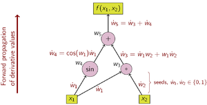
This can be generalized to multiple variables as a matrix product of Jacobians.

Compared to reverse accumulation, forward accumulation is natural and easy to implement as the flow of derivative information coincides with the order of evaluation. Each variable $w$ is augmented with its derivative $ẇ$ (stored as a numerical value, not a symbolic expression),

{\dot {w}}={\frac {\partial w}{\partial x}}

as denoted by the dot. The derivatives are then computed in sync with the evaluation steps and combined with other derivatives via the chain rule.

As an example, consider the function:

{\begin{aligned}z&=f(x_{1},x_{2})\\&=x_{1}x_{2}+\sin x_{1}\\&=w_{1}w_{2}+\sin w_{1}\\&=w_{3}+w_{4}\\&=w_{5}\end{aligned}}

For clarity, the individual sub-expressions have been labeled with the variables

w i

.

The choice of the independent variable to which differentiation is performed affects the seed values $ẇ 1$ and $ẇ 2$ . Given interest in the derivative of this function with respect to $x 1$ , the seed values should be set to:

{\begin{aligned}{\dot {w}}_{1}={\frac {\partial x_{1}}{\partial x_{1}}}=1\\{\dot {w}}_{2}={\frac {\partial x_{2}}{\partial x_{1}}}=0\end{aligned}}

With the seed values set, the values propagate using the chain rule as shown. Figure 2 shows a pictorial depiction of this process as a computational graph.

Operations to compute value	Operations to compute derivative
$w_{1}=x_{1}$	${\dot {w}}_{1}=1$ (seed)
$w_{2}=x_{2}$	${\dot {w}}_{2}=0$ (seed)
$w_{3}=w_{1}\cdot w_{2}$	${\dot {w}}_{3}=w_{2}\cdot {\dot {w}}_{1}+w_{1}\cdot {\dot {w}}_{2}$
$w_{4}=\sin w_{1}$	${\dot {w}}_{4}=\cos w_{1}\cdot {\dot {w}}_{1}$
$w_{5}=w_{3}+w_{4}$	${\dot {w}}_{5}={\dot {w}}_{3}+{\dot {w}}_{4}$

To compute the gradient of this example function, which requires the derivatives of $f$ with respect to not only $x 1$ but also $x 2$ , an additional sweep is performed over the computational graph using the seed values ${\dot {w}}_{1}=0;{\dot {w}}_{2}=1$ .

The computational complexity of one sweep of forward accumulation is proportional to the complexity of the original code.

Forward accumulation is more efficient than reverse accumulation for functions $f : R n \to R m$ with $m ≫ n$ as only $n$ sweeps are necessary, compared to $m$ sweeps for reverse accumulation.

Reverse accumulation[]

Figure 3: Example of reverse accumulation with computational graph

In reverse accumulation AD, the dependent variable to be differentiated is fixed and the derivative is computed with respect to each sub-expression recursively. In a pen-and-paper calculation, the derivative of the outer functions is repeatedly substituted in the chain rule:

{\frac {\partial y}{\partial x}}={\frac {\partial y}{\partial w_{1}}}{\frac {\partial w_{1}}{\partial x}}=\left({\frac {\partial y}{\partial w_{2}}}{\frac {\partial w_{2}}{\partial w_{1}}}\right){\frac {\partial w_{1}}{\partial x}}=\left(\left({\frac {\partial y}{\partial w_{3}}}{\frac {\partial w_{3}}{\partial w_{2}}}\right){\frac {\partial w_{2}}{\partial w_{1}}}\right){\frac {\partial w_{1}}{\partial x}}=\cdots

In reverse accumulation, the quantity of interest is the adjoint, denoted with a bar ( $w̄$ ); it is a derivative of a chosen dependent variable with respect to a subexpression $w$ :

{\bar {w}}={\frac {\partial y}{\partial w}}

Reverse accumulation traverses the chain rule from outside to inside, or in the case of the computational graph in Figure 3, from top to bottom. The example function is scalar-valued, and thus there is only one seed for the derivative computation, and only one sweep of the computational graph is needed to calculate the (two-component) gradient. This is only half the work when compared to forward accumulation, but reverse accumulation requires the storage of the intermediate variables $w i$ as well as the instructions that produced them in a data structure known as a Wengert list (or "tape"),^[3]^[4] which may consume significant memory if the computational graph is large. This can be mitigated to some extent by storing only a subset of the intermediate variables and then reconstructing the necessary work variables by repeating the evaluations, a technique known as rematerialization. Checkpointing is also used to save intermediary states.

The operations to compute the derivative using reverse accumulation are shown in the table below (note the reversed order):

Operations to compute derivative: ${\bar {w}}_{5}=1{\text{ (seed)}}$; ${\bar {w}}_{4}={\bar {w}}_{5}$; ${\bar {w}}_{3}={\bar {w}}_{5}$; ${\bar {w}}_{2}={\bar {w}}_{3}\cdot w_{1}$; ${\bar {w}}_{1}={\bar {w}}_{3}\cdot w_{2}+{\bar {w}}_{4}\cdot \cos w_{1}$

The data flow graph of a computation can be manipulated to calculate the gradient of its original calculation. This is done by adding an adjoint node for each primal node, connected by adjoint edges which parallel the primal edges but flow in the opposite direction. The nodes in the adjoint graph represent multiplication by the derivatives of the functions calculated by the nodes in the primal. For instance, addition in the primal causes fanout in the adjoint; fanout in the primal causes addition in the adjoint;^[a] a unary function $y = f (x)$ in the primal causes $x̄ = ȳ f'(x)$ in the adjoint; etc.

Reverse accumulation is more efficient than forward accumulation for functions $f : R n \to R m$ with $m ≪ n$ as only $m$ sweeps are necessary, compared to $n$ sweeps for forward accumulation.

Reverse mode AD was first published in 1976 by Seppo Linnainmaa.^[5]^[6]

Backpropagation of errors in multilayer perceptrons, a technique used in machine learning, is a special case of reverse mode AD.^[2]

Beyond forward and reverse accumulation[]

Forward and reverse accumulation are just two (extreme) ways of traversing the chain rule. The problem of computing a full Jacobian of $f : R n \to R m$ with a minimum number of arithmetic operations is known as the optimal Jacobian accumulation (OJA) problem, which is NP-complete.^[7] Central to this proof is the idea that algebraic dependencies may exist between the local partials that label the edges of the graph. In particular, two or more edge labels may be recognized as equal. The complexity of the problem is still open if it is assumed that all edge labels are unique and algebraically independent.

Automatic differentiation using dual numbers[]

Forward mode automatic differentiation is accomplished by augmenting the algebra of real numbers and obtaining a new arithmetic. An additional component is added to every number to represent the derivative of a function at the number, and all arithmetic operators are extended for the augmented algebra. The augmented algebra is the algebra of dual numbers.

Replace every number $\,x$ with the number $x+x'\varepsilon$ , where $x'$ is a real number, but $\varepsilon$ is an abstract number with the property $\varepsilon ^{2}=0$ (an infinitesimal; see Smooth infinitesimal analysis). Using only this, regular arithmetic gives

{\begin{aligned}(x+x'\varepsilon )+(y+y'\varepsilon )&=x+y+(x'+y')\varepsilon \\(x+x'\varepsilon )\cdot (y+y'\varepsilon )&=xy+xy'\varepsilon +yx'\varepsilon +x'y'\varepsilon ^{2}=xy+(xy'+yx')\varepsilon \end{aligned}}

and likewise for subtraction and division.

Now, polynomials can be calculated in this augmented arithmetic. If $P(x)=p_{0}+p_{1}x+p_{2}x^{2}+\cdots +p_{n}x^{n}$ , then

{\begin{aligned}P(x+x'\varepsilon )&=p_{0}+p_{1}(x+x'\varepsilon )+\cdots +p_{n}(x+x'\varepsilon )^{n}\\&=p_{0}+p_{1}x+\cdots +p_{n}x^{n}+p_{1}x'\varepsilon +2p_{2}xx'\varepsilon +\cdots +np_{n}x^{n-1}x'\varepsilon \\&=P(x)+P^{(1)}(x)x'\varepsilon \end{aligned}}

where

P^{(1)}

denotes the derivative of

P

with respect to its first argument, and

x'

, called a seed, can be chosen arbitrarily.

The new arithmetic consists of ordered pairs, elements written $\langle x,x'\rangle$ , with ordinary arithmetics on the first component, and first order differentiation arithmetic on the second component, as described above. Extending the above results on polynomials to analytic functions gives a list of the basic arithmetic and some standard functions for the new arithmetic:

{\begin{aligned}\left\langle u,u'\right\rangle +\left\langle v,v'\right\rangle &=\left\langle u+v,u'+v'\right\rangle \\\left\langle u,u'\right\rangle -\left\langle v,v'\right\rangle &=\left\langle u-v,u'-v'\right\rangle \\\left\langle u,u'\right\rangle *\left\langle v,v'\right\rangle &=\left\langle uv,u'v+uv'\right\rangle \\\left\langle u,u'\right\rangle /\left\langle v,v'\right\rangle &=\left\langle {\frac {u}{v}},{\frac {u'v-uv'}{v^{2}}}\right\rangle \quad (v\neq 0)\\\sin \left\langle u,u'\right\rangle &=\left\langle \sin(u),u'\cos(u)\right\rangle \\\cos \left\langle u,u'\right\rangle &=\left\langle \cos(u),-u'\sin(u)\right\rangle \\\exp \left\langle u,u'\right\rangle &=\left\langle \exp u,u'\exp u\right\rangle \\\log \left\langle u,u'\right\rangle &=\left\langle \log(u),u'/u\right\rangle \quad (u>0)\\\left\langle u,u'\right\rangle ^{k}&=\left\langle u^{k},ku^{k-1}u'\right\rangle \quad (u\neq 0)\\\left|\left\langle u,u'\right\rangle \right|&=\left\langle \left|u\right|,u'{\mbox{sign}}u\right\rangle \quad (u\neq 0)\end{aligned}}

and in general for the primitive function

g

,

g(\langle u,u'\rangle ,\langle v,v'\rangle )=\langle g(u,v),g_{u}(u,v)u'+g_{v}(u,v)v'\rangle

where

g_{u}

and

g_{v}

are the derivatives of

g

with respect to its first and second arguments, respectively.

When a binary basic arithmetic operation is applied to mixed arguments—the pair $\langle u,u'\rangle$ and the real number $c$ —the real number is first lifted to $\langle c,0\rangle$ . The derivative of a function $f:\mathbb {R} \to \mathbb {R}$ at the point $x_{0}$ is now found by calculating $f(\langle x_{0},1\rangle )$ using the above arithmetic, which gives $\langle f(x_{0}),f'(x_{0})\rangle$ as the result.

Vector arguments and functions[]

Multivariate functions can be handled with the same efficiency and mechanisms as univariate functions by adopting a directional derivative operator. That is, if it is sufficient to compute $y'=\nabla f(x)\cdot x'$ , the directional derivative $y'\in \mathbb {R} ^{m}$ of $f:\mathbb {R} ^{n}\to \mathbb {R} ^{m}$ at $x\in \mathbb {R} ^{n}$ in the direction $x'\in \mathbb {R} ^{n}$ , this may be calculated as $(\langle y_{1},y'_{1}\rangle ,\ldots ,\langle y_{m},y'_{m}\rangle )=f(\langle x_{1},x'_{1}\rangle ,\ldots ,\langle x_{n},x'_{n}\rangle )$ using the same arithmetic as above. If all the elements of $\nabla f$ are desired, then $n$ function evaluations are required. Note that in many optimization applications, the directional derivative is indeed sufficient.

High order and many variables[]

The above arithmetic can be generalized to calculate second order and higher derivatives of multivariate functions. However, the arithmetic rules quickly grow complicated: complexity is quadratic in the highest derivative degree. Instead, truncated Taylor polynomial algebra can be used. The resulting arithmetic, defined on generalized dual numbers, allows efficient computation using functions as if they were a data type. Once the Taylor polynomial of a function is known, the derivatives are easily extracted.

Implementation[]

Forward-mode AD is implemented by a of the program in which real numbers are replaced by dual numbers, constants are lifted to dual numbers with a zero epsilon coefficient, and the numeric primitives are lifted to operate on dual numbers. This nonstandard interpretation is generally implemented using one of two strategies: source code transformation or operator overloading.

Source code transformation (SCT)[]

Figure 4: Example of how source code transformation could work

The source code for a function is replaced by an automatically generated source code that includes statements for calculating the derivatives interleaved with the original instructions.

Source code transformation can be implemented for all programming languages, and it is also easier for the compiler to do compile time optimizations. However, the implementation of the AD tool itself is more difficult.

Operator overloading (OO)[]

Figure 5: Example of how operator overloading could work

Operator overloading is a possibility for source code written in a language supporting it. Objects for real numbers and elementary mathematical operations must be overloaded to cater for the augmented arithmetic depicted above. This requires no change in the form or sequence of operations in the original source code for the function to be differentiated, but often requires changes in basic data types for numbers and vectors to support overloading and often also involves the insertion of special flagging operations.

Operator overloading for forward accumulation is easy to implement, and also possible for reverse accumulation. However, current compilers lag behind in optimizing the code when compared to forward accumulation.

Operator overloading, for both forward and reverse accumulation, can be well-suited to applications where the objects are vectors of real numbers rather than scalars. This is because the tape then comprises vector operations; this can facilitate computationally efficient implementations where each vector operation performs many scalar operations. Vector adjoint algorithmic differentiation (vector AAD) techniques may be used, for example, to differentiate values calculated by Monte-Carlo simulation.

Examples of operator-overloading implementations of automatic differentiation in C++ are the Adept and Stan libraries.

Notes[]

^ In terms of weight matrices, the adjoint is the transpose. Addition is the covector $[1\cdots 1]$ , since $[1\cdots 1]\left[{\begin{smallmatrix}x_{1}\\\vdots \\x_{n}\end{smallmatrix}}\right]=x_{1}+\cdots +x_{n},$ and fanout is the vector $\left[{\begin{smallmatrix}1\\\vdots \\1\end{smallmatrix}}\right],$ since $\left[{\begin{smallmatrix}1\\\vdots \\1\end{smallmatrix}}\right][x]=\left[{\begin{smallmatrix}x\\\vdots \\x\end{smallmatrix}}\right].$

References[]

^ Neidinger, Richard D. (2010). "Introduction to Automatic Differentiation and MATLAB Object-Oriented Programming" (PDF). SIAM Review. 52 (3): 545–563. CiteSeerX 10.1.1.362.6580. doi:10.1137/080743627.
^ Jump up to: ^a ^b Baydin, Atilim Gunes; Pearlmutter, Barak; Radul, Alexey Andreyevich; Siskind, Jeffrey (2018). "Automatic differentiation in machine learning: a survey". Journal of Machine Learning Research. 18: 1–43.
^ R.E. Wengert (1964). "A simple automatic derivative evaluation program". Comm. ACM. 7 (8): 463–464. doi:10.1145/355586.364791.
^ Bartholomew-Biggs, Michael; Brown, Steven; Christianson, Bruce; Dixon, Laurence (2000). "Automatic differentiation of algorithms". Journal of Computational and Applied Mathematics. 124 (1–2): 171–190. Bibcode:2000JCoAM.124..171B. doi:10.1016/S0377-0427(00)00422-2. hdl:2299/3010.
^ Linnainmaa, Seppo (1976). "Taylor Expansion of the Accumulated Rounding Error". BIT Numerical Mathematics. 16 (2): 146–160. doi:10.1007/BF01931367.
^ Griewank, Andreas (2012). "Who Invented the Reverse Mode of Differentiation?" (PDF). Optimization Stories, Documenta Matematica. Extra Volume ISMP: 389–400.
^ Naumann, Uwe (April 2008). "Optimal Jacobian accumulation is NP-complete". Mathematical Programming. 112 (2): 427–441. CiteSeerX 10.1.1.320.5665. doi:10.1007/s10107-006-0042-z.

External links[]

www.autodiff.org, An "entry site to everything you want to know about automatic differentiation"
Automatic Differentiation of Parallel OpenMP Programs
Automatic Differentiation, C++ Templates and Photogrammetry
Automatic Differentiation, Operator Overloading Approach
Compute analytic derivatives of any Fortran77, Fortran95, or C program through a web-based interface Automatic Differentiation of Fortran programs
Description and example code for forward Automatic Differentiation in Scala
finmath-lib automatic differentiation extensions, Automatic differentiation for random variables (Java implementation of the stochastic automatic differentiation).
Adjoint Algorithmic Differentiation: Calibration and Implicit Function Theorem
C++ Template-based automatic differentiation article and implementation
Tangent Source-to-Source Debuggable Derivatives
[1], Exact First- and Second-Order Greeks by Algorithmic Differentiation
[2], Adjoint Algorithmic Differentiation of a GPU Accelerated Application
[3], Adjoint Methods in Computational Finance Software Tool Support for Algorithmic Differentiationop

[5] In terms of weight matrices, the adjoint is the transpose. Addition is the covector $[1\cdots 1]$ , since $[1\cdots 1]\left[{\begin{smallmatrix}x_{1}\\\vdots \\x_{n}\end{smallmatrix}}\right]=x_{1}+\cdots +x_{n},$ and fanout is the vector $\left[{\begin{smallmatrix}1\\\vdots \\1\end{smallmatrix}}\right],$ since $\left[{\begin{smallmatrix}1\\\vdots \\1\end{smallmatrix}}\right][x]=\left[{\begin{smallmatrix}x\\\vdots \\x\end{smallmatrix}}\right].$

[1] Neidinger, Richard D. (2010). "Introduction to Automatic Differentiation and MATLAB Object-Oriented Programming" (PDF). SIAM Review. 52 (3): 545–563. CiteSeerX 10.1.1.362.6580. doi:10.1137/080743627.

[baydin2018automatic-2] Jump up to: ^a ^b Baydin, Atilim Gunes; Pearlmutter, Barak; Radul, Alexey Andreyevich; Siskind, Jeffrey (2018). "Automatic differentiation in machine learning: a survey". Journal of Machine Learning Research. 18: 1–43.

[3] R.E. Wengert (1964). "A simple automatic derivative evaluation program". Comm. ACM. 7 (8): 463–464. doi:10.1145/355586.364791.

[4] Bartholomew-Biggs, Michael; Brown, Steven; Christianson, Bruce; Dixon, Laurence (2000). "Automatic differentiation of algorithms". Journal of Computational and Applied Mathematics. 124 (1–2): 171–190. Bibcode:2000JCoAM.124..171B. doi:10.1016/S0377-0427(00)00422-2. hdl:2299/3010.

[lin1976-6] Linnainmaa, Seppo (1976). "Taylor Expansion of the Accumulated Rounding Error". BIT Numerical Mathematics. 16 (2): 146–160. doi:10.1007/BF01931367.

[grie2012-7] Griewank, Andreas (2012). "Who Invented the Reverse Mode of Differentiation?" (PDF). Optimization Stories, Documenta Matematica. Extra Volume ISMP: 389–400.

[8] Naumann, Uwe (April 2008). "Optimal Jacobian accumulation is NP-complete". Mathematical Programming. 112 (2): 427–441. CiteSeerX 10.1.1.320.5665. doi:10.1007/s10107-006-0042-z.

[1]

[2]

[3]

[4]

[a]

[5]

[6]

[7]

show Authority control
National libraries	United States
Other	Microsoft Academic