Variational autoencoder

Part of a series on
Machine learning and data mining
Problems Classification Clustering Regression Anomaly detection Data Cleaning AutoML Association rules Reinforcement learning Structured prediction Feature engineering Feature learning Online learning Semi-supervised learning Unsupervised learning Learning to rank Grammar induction
Supervised learning (classification • regression) Decision trees Ensembles Bagging Boosting Random forest k-NN Linear regression Naive Bayes Artificial neural networks Logistic regression Perceptron Relevance vector machine (RVM) Support vector machine (SVM)
Clustering BIRCH CURE Hierarchical k-means Expectation–maximization (EM) DBSCAN OPTICS Mean shift
Dimensionality reduction Factor analysis CCA ICA LDA NMF PCA PGD t-SNE
Structured prediction Graphical models Bayes net Conditional random field Hidden Markov
Anomaly detection k-NN Local outlier factor
Artificial neural network Autoencoder Cognitive computing Deep learning DeepDream Multilayer perceptron RNN LSTM GRU ESN Restricted Boltzmann machine GAN SOM Convolutional neural network U-Net Transformer Vision Spiking neural network Memtransistor Electrochemical RAM (ECRAM)
Reinforcement learning Q-learning SARSA Temporal difference (TD)
Theory Kernel machines Bias–variance tradeoff Computational learning theory Empirical risk minimization Occam learning PAC learning Statistical learning VC theory
Machine-learning venues NeurIPS ICML ML JMLR ArXiv:cs.LG
Related articles Glossary of artificial intelligence List of datasets for machine-learning research Outline of machine learning
v t

In machine learning, a variational autoencoder,^[1] also known as VAE, is the artificial neural network architecture introduced by and Max Welling, belonging to the families of probabilistic graphical models and variational Bayesian methods.

It is often associated with the autoencoder^[2][3] model because of its architectural affinity, but there are significant differences both in the goal and in the mathematical formulation. Variational autoencoders are meant to compress the input information into a constrained multivariate latent distribution (encoding) to reconstruct it as accurately as possible (decoding). Although this type of model was initially designed for unsupervised learning,^[4][5] its effectiveness has been proven in other domains of machine learning such as semi-supervised learning^[6][7] or supervised learning.^[8]

Architecture[]

In a variational autoencoder, the input data is sampled from a parametrized distribution (the prior, in Bayesian inference terms), and the encoder and decoder are trained jointly such that the output minimizes a reconstruction error in the sense of the Kullback-Leibler divergence between the parametric posterior and the true posterior.^[9][10][11]

Formulation[]

The basic scheme of a variational autoencoder. The model receives ${\displaystyle \mathbf {x} }$ as input. The encoder compresses it into the latent space. The decoder receives as input the information sampled from the latent space and produces ${\displaystyle \mathbf {x'} }$ as similar as possible to ${\displaystyle \mathbf {x} }$.

From a formal perspective, given an input dataset ${\displaystyle \mathbf {x} }$ characterized by an unknown probability function ${\displaystyle P(\mathbf {x} )}$ and a multivariate latent encoding vector ${\displaystyle \mathbf {z} }$, the objective is to model the data as a distribution ${\displaystyle p_{\theta }(\mathbf {x} )}$, with ${\displaystyle \theta }$ defined as the set of the network parameters.

It is possible to formalize this distribution as

${\displaystyle p_{\theta }(\mathbf {x} )=\int _{\mathbf {z} }p_{\theta }(\mathbf {x,z} )\,d\mathbf {z} }$

where ${\displaystyle p_{\theta }}$ is the evidence of the model's data with marginalization performed over unobserved variables and thus ${\displaystyle p_{\theta }(\mathbf {x,z} )}$ represents the joint distribution between input data and its latent representation according to the network parameters ${\displaystyle \theta }$.

According to the chain rule, the equation can be rewritten as

${\displaystyle p_{\theta }(\mathbf {x} )=\int _{\mathbf {z} }p_{\theta }(\mathbf {x\mid z} )p_{\theta }(\mathbf {z} )\,d\mathbf {z} }$

In the vanilla variational autoencoder we assume ${\displaystyle \mathbf {z} }$ with finite dimension and that ${\displaystyle p_{\theta }(\mathbf {x|z} )}$ is a Gaussian distribution, then ${\displaystyle p_{\theta }(\mathbf {x} )}$ is a mixture of Gaussian distributions.

It is now possible to define the set of the relationships between the input data and its latent representation as

• Prior ${\displaystyle p_{\theta }(\mathbf {z} )}$
• Likelihood ${\displaystyle p_{\theta }(\mathbf {x} \mid \mathbf {z} )}$
• Posterior ${\displaystyle p_{\theta }(\mathbf {z} \mid \mathbf {x} )}$

Unfortunately, the computation of ${\displaystyle p_{\theta }(\mathbf {x} )}$ is very expensive and in most cases even intractable. To speed up the calculus and make it feasible, it is necessary to introduce a further function to approximate the posterior distribution as

${\displaystyle q_{\Phi }(\mathbf {z\mid x} )\approx p_{\theta }(\mathbf {z\mid x} )}$

with ${\displaystyle \Phi }$ defined as the set of real values that parametrize ${\displaystyle q}$.

In this way, the overall problem can be easily translated into the autoencoder domain, in which the conditional likelihood distribution ${\displaystyle p_{\theta }(\mathbf {x} \mid \mathbf {z} )}$ is carried by the probabilistic decoder, while the approximated posterior distribution ${\displaystyle q_{\Phi }(\mathbf {z} \mid \mathbf {x} )}$ is computed by the probabilistic encoder.

ELBO loss function[]

As in every deep learning problem, it is necessary to define a differentiable loss function in order to update the network weights through backpropagation.

For variational autoencoders the idea is to jointly minimize the generative model parameters ${\displaystyle \theta }$ to reduce the reconstruction error between the input and the output of the network, and ${\displaystyle \Phi }$ to have ${\displaystyle q_{\Phi }(\mathbf {z\mid x} )}$ as close as possible to ${\displaystyle p_{\theta }(\mathbf {z} \mid \mathbf {x} )}$.

As reconstruction loss, mean squared error and cross entropy represent good alternatives.

As distance loss between the two distributions the reverse Kullback–Leibler divergence ${\displaystyle D_{KL}(q_{\Phi }(\mathbf {z\mid x} )\parallel p_{\theta }(\mathbf {z\mid x} ))}$ is a good choice to squeeze ${\displaystyle q_{\Phi }(\mathbf {z\mid x} )}$ under ${\displaystyle p_{\theta }(\mathbf {z} \mid \mathbf {x} )}$.^[1][12]

The distance loss just defined is expanded as

${\displaystyle {\begin{aligned}D_{KL}(q_{\Phi }(\mathbf {z\mid x} )\parallel p_{\theta }(\mathbf {z\mid x} ))&=\int q_{\Phi }(\mathbf {z\mid x} )\log {\frac {q_{\Phi }(\mathbf {z\mid x} )}{p_{\theta }(\mathbf {z\mid x} )}}\,d\mathbf {z} \\&=\int q_{\Phi }(\mathbf {z\mid x} )\log {\frac {q_{\Phi }(\mathbf {z\mid x} )p_{\theta }(\mathbf {x} )}{p_{\theta }(\mathbf {z,x} )}}\,d\mathbf {z} \\&=\int q_{\Phi }(\mathbf {z\mid x} )\left(\log(p_{\theta }(\mathbf {x} ))+\log {\frac {q_{\Phi }(\mathbf {z\mid x} )}{p_{\theta }(\mathbf {z,x} )}}\right)d\mathbf {z} \\&=\log(p_{\theta }(\mathbf {x} ))+\int q_{\Phi }(\mathbf {z\mid x} )\log {\frac {q_{\Phi }(\mathbf {z\mid x} )}{p_{\theta }(\mathbf {z,x} )}}\,d\mathbf {z} \\&=\log(p_{\theta }(\mathbf {x} ))+\int q_{\Phi }(\mathbf {z\mid x} )\log {\frac {q_{\Phi }(\mathbf {z\mid x} )}{p_{\theta }(\mathbf {x\mid z} )p_{\theta }(\mathbf {z} )}}\,d\mathbf {z} \\&=\log(p_{\theta }(\mathbf {x} ))+E_{\mathbf {z} \sim q_{\Phi }(\mathbf {z\mid x} )}(\log {\frac {q_{\Phi }(\mathbf {z\mid x} )}{p_{\theta }(\mathbf {z} )}}-\log(p_{\theta }(\mathbf {x\mid z} )))\\&=\log(p_{\theta }(\mathbf {x} ))+D_{KL}(q_{\Phi }(\mathbf {z\mid x} )\parallel p_{\theta }(\mathbf {z} ))-E_{\mathbf {z} \sim q_{\Phi }(\mathbf {z\mid x} )}(\log(p_{\theta }(\mathbf {x\mid z} )))\end{aligned}}}$

At this point, it is possible to rewrite the equation as

${\displaystyle \log(p_{\theta }(\mathbf {x} ))-D_{KL}(q_{\Phi }(\mathbf {z\mid x} )\parallel p_{\theta }(\mathbf {z\mid x} ))=E_{\mathbf {z} \sim q_{\Phi }(\mathbf {z\mid x} )}(\log(p_{\theta }(\mathbf {x\mid z} )))-D_{KL}(q_{\Phi }(\mathbf {z\mid x} )\parallel p_{\theta }(\mathbf {z} ))}$

The goal is to maximize the log-likelihood of the LHS of the equation to improve the generated data quality and to minimize the distribution distances between the real posterior and the estimated one.

This is equivalent to minimize the negative log-likelihood, which is a common practice in optimization problems.

The loss function so obtained, also named evidence lower bound loss function, shortly ELBO, can be written as

${\displaystyle L_{\theta ,\Phi }=-\log(p_{\theta }(\mathbf {x} ))+D_{KL}(q_{\Phi }(\mathbf {z\mid x} )\parallel p_{\theta }(\mathbf {z\mid x} ))=-E_{\mathbf {z} \sim q_{\Phi }(\mathbf {z|x} )}(\log(p_{\theta }(\mathbf {x\mid z} )))+D_{KL}(q_{\Phi }(\mathbf {z\mid x} )\parallel p_{\theta }(\mathbf {z} ))}$

Given the non-negative property of the Kullback–Leibler divergence, it is correct to assert that

${\displaystyle -L_{\theta ,\Phi }=\log(p_{\theta }(\mathbf {x} ))-D_{KL}(q_{\Phi }(\mathbf {z\mid x} )\parallel p_{\theta }(\mathbf {z\mid x} ))\leq \log(p_{\theta }(\mathbf {x} ))}$

The optimal parameters are the ones that minimize this loss function. The problem can be summarized as

${\displaystyle \theta ^{*},\Phi ^{*}={\underset {\theta ,\Phi }{\operatorname {argmin} }}\,L_{\theta ,\Phi }}$

The main advantage of this formulation relies on the possibility to jointly optimize with respect to parameters ${\displaystyle \theta }$ and ${\displaystyle \Phi }$.

Before applying the ELBO loss function to an optimization problem to backpropagate the gradient, it is necessary to make it differentiable by applying the so-called reparameterization trick to remove the stochastic sampling from the formation, and thus making it differentiable.

Reparameterization trick[]

The scheme of the reparameterization trick. The randomness variable ${\displaystyle \mathbf {\varepsilon } }$ is injected into the latent space ${\displaystyle \mathbf {z} }$ as external input. In this way, it is possible to backpropagate the gradient without involving stochastic variable during the update.

To make the ELBO formulation suitable for training purposes, it is necessary to introduce a further minor modification to the formulation of the problem and as well as to the structure of the variational autoencoder.^[1][13][14]

Stochastic sampling is the non-differentiable operation through which it is possible to sample from the latent space and feed the probabilistic decoder.

In order to make the application of backpropagation processes feasible, such as the stochastic gradient descent, the reparameterization trick is introduced.

The main assumption about the latent space is that it can be considered as a set of multivariate Gaussian distributions, and thus can be described as

${\displaystyle \mathbf {z} \sim q_{\Phi }(\mathbf {z} \mid \mathbf {x} )={\mathcal {N}}({\boldsymbol {\mu }},{\boldsymbol {\sigma }}^{2})}$

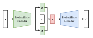The scheme of a variational autoencoder after the reparameterization trick.

Given ${\displaystyle {\boldsymbol {\varepsilon }}\sim {\mathcal {N}}(0,{\boldsymbol {I}})}$ and ${\displaystyle \odot }$ defined as the element-wise product, the reparameterization trick modifies the above equation as

${\displaystyle \mathbf {z} ={\boldsymbol {\mu }}+{\boldsymbol {\sigma }}\odot {\boldsymbol {\varepsilon }}.}$

Thanks to this transformation, that can be extended also to other distributions different from the Gaussian, the variational autoencoder is trainable and the probabilistic encoder has to learn how to map a compressed representation of the input into the two latent vectors ${\displaystyle {\boldsymbol {\mu }}}$ and ${\displaystyle {\boldsymbol {\sigma }}}$, while the stochasticity remains excluded from the updating process and is injected in the latent space as an external input through the random vector ${\displaystyle {\boldsymbol {\varepsilon }}}$.

Variations[]

There are many variational autoencoders applications and extensions in order to adapt the architecture to different domains and improve its performance.

${\displaystyle \beta }$-VAE is an implementation with a weighted Kullback–Leibler divergence term to automatically discover and interpret factorised latent representations. With this implementation, it is possible to force manifold disentanglement for ${\displaystyle \beta }$ values greater than one. The authors demonstrate this architecture ability to generate high-quality synthetic samples.^[15][16]

One other implementation named conditional variational autoencoder, shortly CVAE, is thought to insert label information in the latent space so to force a deterministic constrained representation of the learned data.^[17]

Some structures directly deal with the quality of the generated samples^[18][19] or implement more than one latent space to further improve the representation learning.^[20][21]

Some architectures mix the structures of variational autoencoders and generative adversarial networks to obtain hybrid models with high generative capabilities.^[22][23][24]

See also[]

References[]