Pacific decadal oscillation
This article has multiple issues. Please help or discuss these issues on the talk page. (Learn how and when to remove these template messages)
|
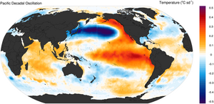
The Pacific decadal oscillation (PDO) is a robust, recurring pattern of ocean-atmosphere climate variability centered over the mid-latitude Pacific basin. The PDO is detected as warm or cool surface waters in the Pacific Ocean, north of 20°N. Over the past century, the amplitude of this climate pattern has varied irregularly at interannual-to-interdecadal time scales (meaning time periods of a few years to as much as time periods of multiple decades). There is evidence of reversals in the prevailing polarity (meaning changes in cool surface waters versus warm surface waters within the region) of the oscillation occurring around 1925, 1947, and 1977; the last two reversals corresponded with dramatic shifts in salmon production regimes in the North Pacific Ocean. This climate pattern also affects coastal sea and continental surface air temperatures from Alaska to California.
During a "warm", or "positive", phase, the west Pacific becomes cooler and part of the eastern ocean warms; during a "cool", or "negative", phase, the opposite pattern occurs. The Pacific decadal oscillation was named by Steven R. Hare, who noticed it while studying salmon production pattern results in 1997.[1]
The Pacific decadal oscillation index is the leading empirical orthogonal function (EOF) of monthly sea surface temperature anomalies (SST-A) over the North Pacific (poleward of 20°N) after the global average sea surface temperature has been removed. This PDO index is the standardized principal component time series.[2] A PDO 'signal' has been reconstructed as far back as 1661 through tree-ring chronologies in the Baja California area.[3]
Mechanisms[]
Several studies have indicated that the PDO index can be reconstructed as the superimposition of tropical forcing and extra-tropical processes.[4][5][6][7] Thus, unlike El Niño–Southern Oscillation (ENSO), the PDO is not a single physical mode of ocean variability, but rather the sum of several processes with different dynamic origins.
At inter-annual time scales the PDO index is reconstructed as the sum of random and ENSO induced variability in the Aleutian Low, whereas on decadal timescales ENSO teleconnections, stochastic atmospheric forcing and changes in the North Pacific oceanic gyre circulation contribute approximately equally. Additionally sea surface temperature anomalies have some winter to winter persistence due to the reemergence mechanism.
- ENSO teleconnections, the atmospheric bridge[8]

ENSO can influence the global circulation pattern thousands of kilometers away from the equatorial Pacific through the "atmospheric bridge". During El Niño events, deep convection and heat transfer to the troposphere is enhanced over the anomalously warm sea surface temperature, this ENSO-related tropical forcing generates Rossby waves that propagate poleward and eastward and are subsequently refracted back from the pole to the tropics. The planetary waves form at preferred locations both in the North and South Pacific Ocean, and the teleconnection pattern is established within 2–6 weeks.[9] ENSO driven patterns modify surface temperature, humidity, wind, and the distribution of clouds over the North Pacific that alter surface heat, momentum, and freshwater fluxes and thus induce sea surface temperature, salinity, and mixed layer depth (MLD) anomalies.
The atmospheric bridge is more effective during boreal winter when the deepened Aleutian Low results in stronger and cold northwesterly winds over the central Pacific and warm/humid southerly winds along the North American west coast, the associated changes in the surface heat fluxes and to a lesser extent Ekman transport creates negative sea surface temperature anomalies and a deepened MLD in the central Pacific and warm the ocean from the Hawaii to the Bering Sea.
- SST reemergence[10]


Midlatitude SST anomaly patterns tend to recur from one winter to the next but not during the intervening summer, this process occurs because of the strong mixed layer seasonal cycle. The mixed layer depth over the North Pacific is deeper, typically 100-200m, in winter than it is in summer and thus SST anomalies that form during winter and extend to the base of the mixed layer are sequestered beneath the shallow summer mixed layer when it reforms in late spring and are effectively insulated from the air-sea heat flux. When the mixed layer deepens again in the following autumn/early winter the anomalies may again influence the surface. This process has been named "reemergence mechanism" by Alexander and Deser[11] and is observed over much of the North Pacific Ocean although it is more effective in the west where the winter mixed layer is deeper and the seasonal cycle greater.
- Stochastic atmospheric forcing[12]
Long term sea surface temperature variation may be induced by random atmospheric forcings that are integrated and reddened into the ocean mixed layer. The stochastic climate model paradigm was proposed by Frankignoul and Hasselmann,[13] in this model a stochastic forcing represented by the passage of storms alter the ocean mixed layer temperature via surface energy fluxes and Ekman currents and the system is damped due to the enhanced (reduced) heat loss to the atmosphere over the anomalously warm (cold) SST via turbulent energy and longwave radiative fluxes, in the simple case of a linear negative feedback the model can be written as the separable ordinary differential equation:

where v is the random atmospheric forcing, λ is the damping rate (positive and constant) and y is the response.
The variance spectrum of y is:

where F is the variance of the white noise forcing and w is the frequency, an implication of this equation is that at short time scales (w>>λ) the variance of the ocean temperature increase with the square of the period while at longer timescales(w<<λ, ~150 months) the damping process dominates and limits sea surface temperature anomalies so that the spectra became white.
Thus an atmospheric white noise generates SST anomalies at much longer timescales but without spectral peaks. Modeling studies suggest that this process contribute to as much as 1/3 of the PDO variability at decadal timescales.
- Ocean dynamics
Several dynamic oceanic mechanisms and SST-air feedback may contribute to the observed decadal variability in the North Pacific Ocean. SST variability is stronger in the Kuroshio Oyashio extension (KOE) region and is associated with changes in the KOE axis and strength,[7] that generates decadal and longer time scales SST variance but without the observed magnitude of the spectral peak at ~10 years, and SST-air feedback. Remote reemergence occurs in regions of strong current such as the Kuroshio extension and the anomalies created near the Japan may reemerge the next winter in the central pacific.
- Advective resonance
Saravanan and McWilliams[14] have demonstrated that the interaction between spatially coherent atmospheric forcing patterns and an advective ocean shows periodicities at preferred time scales when non-local advective effects dominate over the local sea surface temperature damping. This "advective resonance" mechanism may generate decadal SST variability in the Eastern North Pacific associated with the anomalous Ekman advection and surface heat flux.[15]
- North Pacific oceanic gyre circulation
Dynamic gyre adjustments are essential to generate decadal SST peaks in the North Pacific, the process occurs via westward propagating oceanic Rossby waves that are forced by wind anomalies in the central and eastern Pacific Ocean. The quasi-geostrophic equation for long non-dispersive Rossby Waves forced by large scale wind stress can be written as the linear partial differential equation:[16]

where h is the upper-layer thickness anomaly, τ is the wind stress, c is the Rossby wave speed that depends on latitude, ρ0 is the density of sea water and f0 is the Coriolis parameter at a reference latitude. The response time scale is set by the Rossby waves speed, the location of the wind forcing and the basin width, at the latitude of the Kuroshio Extension c is 2.5 cm s−1 and the dynamic gyre adjustment timescale is ~(5)10 years if the Rossby wave was initiated in the (central)eastern Pacific Ocean.
If the wind white forcing is zonally uniform it should generate a red spectrum in which h variance increases with the period and reaches a constant amplitude at lower frequencies without decadal and interdecadal peaks, however low frequencies atmospheric circulation tends to be dominated by fixed spatial patterns so that wind forcing is not zonally uniform, if the wind forcing is zonally sinusoidal then decadal peaks occurs due to resonance of the forced basin-scale Rossby waves.
The propagation of h anomalies in the western pacific changes the KOE axis and strength[7] and impact SST due to the anomalous geostrophic heat transport. Recent studies[7][17] suggest that Rossby waves excited by the Aleutian low propagate the PDO signal from the North Pacific to the KOE through changes in the KOE axis while Rossby waves associated with the NPO propagate the North Pacific Gyre oscillation signal through changes in the KOE strength.
Impacts[]
Temperature and precipitation


The PDO spatial pattern and impacts are similar to those associated with ENSO events. During the positive phase the wintertime Aleutian Low is deepened and shifted southward, warm/humid air is advected along the North American west coast and temperatures are higher than usual from the Pacific Northwest to Alaska but below normal in Mexico and the Southeastern United States.[18]
Winter precipitation is higher than usual in the Alaska Coast Range, Mexico and the Southwestern United States but reduced over Canada, Eastern Siberia and Australia[18][19]
McCabe et al.[20] showed that the PDO along with the AMO strongly influence multidecadal droughts pattern in the United States, drought frequency is enhanced over much of the Northern United States during the positive PDO phase and over the Southwest United States during the negative PDO phase in both cases if the PDO is associated with a positive AMO.
The Asian Monsoon is also affected, increased rainfall and decreased summer temperature is observed over the Indian subcontinent during the negative phase.[21]
| PDO Indicators | PDO positive phase | PDO negative phase |
|---|---|---|
| Temperature | ||
| Pacific Northwest, British Columbia, and Alaska | Above average | Below average |
| Mexico to South-East US | Below average | Above average |
| Precipitation | ||
| Alaska coastal range | Above average | Below average |
| Mexico to South-Western US | Above average | Below average |
| Canada, Eastern Siberia and Australia | Below average | Above average |
| India summer monsoon | Below average | Above average |
Reconstructions and regime shifts[]


The PDO index has been reconstructed using tree rings and other hydrologically sensitive proxies from west North America and Asia.[3][22][23]
MacDonald and Case[24] reconstructed the PDO back to 993 using tree rings from California and Alberta. The index shows a 50–70 year periodicity but is a strong mode of variability only after 1800, a persistent negative phase occurring during medieval times (993–1300) which is consistent with La Niña conditions reconstructed in the tropical Pacific[25] and multi-century droughts in the South-West United States.[26]
Several regime shifts are apparent both in the reconstructions and instrumental data, during the 20th century regime shifts associated with concurrent changes in SST, SLP, land precipitation and ocean cloud cover occurred in 1924/1925, 1945/1946, and 1976/1977:[27]
- 1750: PDO displays an unusually strong oscillation.[3]
- 1924/1925: PDO changed to a "warm" phase.[27]
- 1945/1946: The PDO changed to a "cool" phase, the pattern of this regime shift is similar to the 1970s episode with maximum amplitude in the subarctic and subtropical front but with a greater signature near the Japan while the 1970s shift was stronger near the American west coast.[27][28]
- 1976/1977: PDO changed to a "warm" phase.[29]
- 1988/1989: A weakening of the Aleutian low with associated SST changes was observed,[30] in contrast to others regime shifts this change appears to be related to concurrent extratropical oscillation in the North Pacific and North Atlantic rather than tropical processes.[31]
- 1997/1998: Several changes in sea surface temperature and marine ecosystem occurred in the North Pacific after 1997/1998, in contrast to prevailing anomalies observed after the 1970s shift. The SST declined along the United States west coast and substantial changes in the populations of salmon, anchovy and sardine were observed as the PDO changed back to a cool "anchovy" phase.[32] However the spatial pattern of the SST change was different with a meridional SST seesaw in the central and western Pacific that resembled a strong shift in the North Pacific Gyre Oscillation rather than the PDO structure. This pattern dominated much of the North Pacific SST variability after 1989.[33]
- The 2014 flip from the cool PDO phase to the warm phase, which vaguely resembles a long and drawn-out El Niño event, contributed to record-breaking surface temperatures across the planet in 2014.
Predictability[]
The NOAA Earth System Research Laboratory produces official ENSO forecasts, and Experimental statistical forecasts using a linear inverse modeling (LIM) method[34][35] to predict the PDO, LIM assumes that the PDO can be separated into a linear deterministic component and a non-linear component represented by random fluctuations.
Much of the LIM PDO predictability arises from ENSO and the global trend rather than extra-tropical processes and is thus limited to ~4 seasons. The prediction is consistent with the seasonal footprinting mechanism[36] in which an optimal SST structure evolves into the ENSO mature phase 6–10 months later that subsequently impacts the North Pacific Ocean SST via the atmospheric bridge.
Skills in predicting decadal PDO variability could arise from taking into account the impact of the externally forced[37] and internally generated[38] Pacific variability.
Related patterns[]
- The interdecadal Pacific oscillation (IPO) is a similar but less localised phenomenon; it covers the Southern hemisphere as well (50°S to 50°N).
- ENSO tends to lead PDO cycling.
- Shifts in the IPO change the location and strength of ENSO activity. The South Pacific convergence zone moves northeast during El Niño and southwest during La Niña events. The same movement takes place during positive IPO and negative IPO phases respectively. (Folland et al., 2002)
- Interdecadal temperature variations in China are closely related to those of the NAO and the NPO.
- The amplitudes of the NAO and NPO increased in the 1960s and interannual variation patterns changed from 3–4 years to 8–15 years.
- Sea level rise is affected when large areas of water warm and expand, or cool and contract.
See also[]
- California Current
- Hadley cell
- Ocean heat content
- Pacific–North American teleconnection pattern
- North Atlantic oscillation
- Atlantic multidecadal oscillation (AMO)
References[]
- ^ Mantua, Nathan J.; Hare, Steven R.; Zhang, Yuan; Wallace, John M.; Francis, Robert C. (1997). "A Pacific interdecadal climate oscillation with impacts on salmon production". Bulletin of the American Meteorological Society. 78 (6): 1069–79. Bibcode:1997BAMS...78.1069M. doi:10.1175/1520-0477(1997)078<1069:APICOW>2.0.CO;2.
- ^ Deser, Clara; Alexander, Michael A.; Xie, Shang-Ping; Phillips, Adam S. (January 2010). "Sea Surface Temperature Variability: Patterns and Mechanisms". Annual Review of Marine Science. 2 (1): 115–143. Bibcode:2010ARMS....2..115D. doi:10.1146/annurev-marine-120408-151453. PMID 21141660.
- ^ a b c Biondi, Franco; Gershunov, Alexander; Cayan, Daniel R. (2001). "North Pacific Decadal Climate Variability since 1661". Journal of Climate. 14 (1): 5–10. Bibcode:2001JCli...14....5B. doi:10.1175/1520-0442(2001)014<0005:NPDCVS>2.0.CO;2.
- ^ Newman, M.; Compo, G.P.; Alexander, Michael A. (2003). "ENSO-Forced Variability of the Pacific Decadal Oscillation". Journal of Climate. 16 (23): 3853–7. Bibcode:2003JCli...16.3853N. doi:10.1175/1520-0442(2003)016<3853:EVOTPD>2.0.CO;2. S2CID 17779179.
- ^ Vimont, Daniel J. (2005). "The Contribution of the Interannual ENSO Cycle to the Spatial Pattern of Decadal ENSO-Like Variability". Journal of Climate. 18 (12): 2080–92. Bibcode:2005JCli...18.2080V. doi:10.1175/JCLI3365.1.
- ^ Schneider, Niklas; Bruce D. Cornuelle (2005). "The Forcing of the Pacific Decadal Oscillation". Journal of Climate. 18 (8): 4355–72. Bibcode:2005JCli...18.4355S. doi:10.1175/JCLI3527.1.
- ^ a b c d Qiu, Bo; Niklas Schneider; Shuiming Chen (2007). "Coupled Decadal Variability in the North Pacific: An Observationally Constrained Idealized Model". Journal of Climate. 20 (14): 3602–20. Bibcode:2007JCli...20.3602Q. doi:10.1175/JCLI4190.1.
- ^ Alexander, Michael A; Ileana Bladé; Matthew Newman; John R. Lanzante; Ngar-Cheung Lau; James D. Scott (2002). "The Atmospheric Bridge: The Influence of ENSO Teleconnections on Air–Sea Interaction over the Global Oceans". Journal of Climate. 15 (16): 2205–31. Bibcode:2002JCli...15.2205A. doi:10.1175/1520-0442(2002)015<2205:TABTIO>2.0.CO;2.
- ^ Liu, Zhengyu; Alexander Michael (2007). "Atmospheric bridge, oceanic tunnel, and global climate teleconnections". Reviews of Geophysics. 45 (2): 2. Bibcode:2007RvGeo..45.2005L. doi:10.1029/2005RG000172.
- ^ Deser, Clara; Michael A. Alexander; Michael S. Timlin (2003). "Understanding the Persistence of Sea Surface Temperature Anomalies in Midlatitudes". Journal of Climate. 16 (12): 57–72. Bibcode:2003JCli...16...57D. doi:10.1175/1520-0442(2003)016<0057:UTPOSS>2.0.CO;2.
- ^ Alexander, Michael A.; Deser Clara (1995). "A Mechanism for the Recurrence of Wintertime Midlatitude SST Anomalies". Journal of Physical Oceanography. 125 (1): 122–137. Bibcode:1995JPO....25..122A. doi:10.1175/1520-0485(1995)025<0122:AMFTRO>2.0.CO;2.
- ^ Alexander, Michael A.; Penland, Cecile (1996). "Variability in a mixed layer ocean model driven by stochastic atmospheric forcing". Journal of Climate. 9 (10): 2424–42. Bibcode:1996JCli....9.2424A. doi:10.1175/1520-0442(1996)009<2424:VIAMLO>2.0.CO;2.
- ^ Frankignoul, Claude; Hasselmann, Klaus (1977). "Stochastic climate models, Part II Application to sea-surface temperature anomalies and thermocline variability". Tellus. 24 (4): 289–305. Bibcode:1977TellA..29..289F. doi:10.1111/j.2153-3490.1977.tb00740.x.
- ^ Saravanan, R.; McWilliams James C. (1998). "Advective Ocean–Atmosphere Interaction: An Analytical Stochastic Model with Implications for Decadal Variability". Journal of Climate. 11 (2): 165–188. Bibcode:1998JCli...11..165S. doi:10.1175/1520-0442(1998)011<0165:AOAIAA>2.0.CO;2.
- ^ Wu, Lixin; Zhengyu Liu (2003). "Decadal Variability in the North Pacific: The Eastern North Pacific Mode". Journal of Climate. 16 (19): 3111–31. Bibcode:2003JCli...16.3111W. doi:10.1175/1520-0442(2003)016<3111:DVITNP>2.0.CO;2.
- ^ Jin, Fei-Fei (1997). "A Theory of Interdecadal Climate Variability of the North Pacific Ocean–Atmosphere System". Journal of Climate. 10 (8): 1821–35. Bibcode:1997JCli...10.1821J. doi:10.1175/1520-0442(1997)010<1821:ATOICV>2.0.CO;2.
- ^ Ceballos, Lina; Lorenzo, Emanuele Di; Hoyos, Carlos D.; Schneider, Niklas; Taguchi, Bunmei (2009). "North Pacific Gyre Oscillation Synchronizes Climate Fluctuations in the Eastern and Western Boundary Systems". Journal of Climate. 22 (19): 5163–74. Bibcode:2009JCli...22.5163C. doi:10.1175/2009JCLI2848.1.
- ^ a b Mantua, Nathan J.; Hare, Steven R. (1 January 2002). "The Pacific Decadal Oscillation" (PDF). Journal of Oceanography. 58 (1): 35–44. doi:10.1023/A:1015820616384. S2CID 5307916. Archived from the original (PDF) on 8 January 2016. Retrieved 24 May 2013.
- ^ Power, S.; et al. (1998). "Australian temperature, Australian rainfall and the Southern Oscillation, 1910-1992: coherent variability and recent changes" (PDF). Australian Meteorological Magazine. 47 (2): 85–101. Retrieved 8 April 2013.[permanent dead link]
- ^ McCabe, G. J.; Palecki, M. A.; Betancourt, J. L. (11 March 2004). "Pacific and Atlantic Ocean influences on multidecadal drought frequency in the United States". Proceedings of the National Academy of Sciences. 101 (12): 4136–41. Bibcode:2004PNAS..101.4136M. doi:10.1073/pnas.0306738101. PMC 384707. PMID 15016919.
- ^ Krishnan, R.; Sugi, M. (31 August 2003). "Pacific decadal oscillation and variability of the Indian summer monsoon rainfall". Climate Dynamics. 21 (3–4): 233–242. Bibcode:2003ClDy...21..233K. doi:10.1007/s00382-003-0330-8. S2CID 140557286.
- ^ Shen, Caiming; Wei-Chyung Wang; Wei Gong; Zhixin Hao (2006). "A Pacific Decadal Oscillation record since 1470 AD reconstructed from proxy data of summer rainfall over eastern China". Geophys. Res. Lett. 33 (3): L03702. Bibcode:2006GeoRL..33.3702S. doi:10.1029/2005GL024804.
- ^ D'arrigo, R.; Wilson R. (2006). "On the Asian Expression of the PDO". International Journal of Climatology. 26 (12): 1607–17. Bibcode:2006IJCli..26.1607D. doi:10.1002/joc.1326.
- ^ MacDonald, G.M.; Case R.A. (2005). "Variations in the Pacific Decadal Oscillation over the past millennium". Geophys. Res. Lett. 32 (8): L08703. Bibcode:2005GeoRL..32.8703M. doi:10.1029/2005GL022478. Retrieved 2010-10-26.
- ^ Rein, Bert; Andreas Lückge; Frank Sirocko (2004). "AA major Holocene ENSO anomaly during the Medieval period". Geophys. Res. Lett. 31 (17): n/a. Bibcode:2004GeoRL..3117211R. doi:10.1029/2004GL020161. Retrieved 2010-10-26.
- ^ Seager, Richard; Graham, Nicholas; Herweijer, Celine; Gordon, Arnold L.; Kushnir, Yochanan; Cook, Ed (2007). "Blueprints for Medieval hydroclimate" (PDF). Quaternary Science Reviews. 26 (19–21): 2322–36. Bibcode:2007QSRv...26.2322S. doi:10.1016/j.quascirev.2007.04.020.
- ^ a b c Deser, Clara; Phillips, Adam S.; Hurrell, James W. (2004). "Pacific Interdecadal Climate Variability: Linkages between the Tropics and the North Pacific during Boreal Winter since 1900". Journal of Climate. 17 (15): 3109–24. Bibcode:2004JCli...17.3109D. doi:10.1175/1520-0442(2004)017<3109:PICVLB>2.0.CO;2. S2CID 6868642.
- ^ Minobe, Shoshiro; Atsushi Maeda (2005). "A 1° monthly gridded sea-surface temperature dataset compiled from ICOADS from 1850 to 2002 and Northern Hemisphere frontal variability". International Journal of Climatology. 25 (7): 881–894. Bibcode:2005IJCli..25..881M. doi:10.1002/joc.1170.
- ^ Hare, Steven R.; Mantua, Nathan J. (2000). "Empirical evidence for North Pacific regime shifts in 1977 and 1989". Progress in Oceanography. 47 (2–4): 103–145. Bibcode:2000PrOce..47..103H. doi:10.1016/S0079-6611(00)00033-1.
- ^ Trenberth, Kevin; Hurrell, James W. (1994). "Decadal atmosphere-ocean variations in the Pacific". Climate Dynamics. 9 (6): 303–319. Bibcode:1994ClDy....9..303T. doi:10.1007/BF00204745. S2CID 15783178.
- ^ Yasunaka, Sayaka; Kimio Hanawa (2003). "Regime Shifts in the Northern Hemisphere SST Field: Revisited in Relation to Tropical Variations". Journal of the Meteorological Society of Japan. 81 (2): 415–424. doi:10.2151/jmsj.81.415.
- ^ Chavez, Francisco P; Ryan, John; Lluch-Cota, Salvador E.; Ñiquen C., Miguel (2003). "From Anchovies to Sardines and Back: Multidecadal Change in the Pacific Ocean". Science. 299 (5604): 217–221. Bibcode:2003Sci...299..217C. doi:10.1126/science.1075880. PMID 12522241. S2CID 37990897.
- ^ Bond, N.A.; J. E. Overland; M. Spillane; P. Stabeno (2003). "Recent shifts in the state of the North Pacific". Geophys. Res. Lett. 30 (23): n/a. Bibcode:2003GeoRL..30.2183B. doi:10.1029/2003GL018597.
- ^ Team, ESRL Web. "ESRL PSD : ENSO Forecasts". NOAA Earth System Research Laboratory. Retrieved 27 August 2016.
- ^ Alexander, Michael A.; Ludmila Matrosova; Cécile Penland; James D. Scott; Ping Chang (2008). "Forecasting Pacific SSTs: Linear Inverse Model Predictions of the PDO" (PDF). Journal of Climate. 21 (2): 385–402. Bibcode:2008JCli...21..385A. CiteSeerX 10.1.1.639.3207. doi:10.1175/2007JCLI1849.1.
- ^ Vimont, Daniel J.; John M. Wallace; David S. Battisti (2003). "The Seasonal Footprinting Mechanism in the Pacific: Implications for ENSO". Journal of Climate. 16 (16): 2668–75. Bibcode:2003JCli...16.2668V. doi:10.1175/1520-0442(2003)016<2668:TSFMIT>2.0.CO;2. S2CID 131608480.
- ^ Meehl, Gerard A.; Aixue Hu; Benjamin D. Santer (2009). "The Mid-1970s Climate Shift in the Pacific and the Relative Roles of Forced versus Inherent Decadal Variability". Journal of Climate. 22 (3): 780–792. Bibcode:2009JCli...22..780M. doi:10.1175/2008JCLI2552.1. S2CID 15189469.
- ^ Mochizuki, Takashi; Ishii, Masayoshi; Kimoto, Masahide; Chikamotoc, Yoshimitsu; Watanabec, Masahiro; Nozawad, Toru; Sakamotoa, Takashi T.; Shiogamad, Hideo; Awajia, Toshiyuki; Sugiuraa, Nozomi; Toyodaa, Takahiro; Yasunakac, Sayaka; Tatebea, Hiroaki; Moric, Masato (2010). "Pacific decadal oscillation hindcasts relevant to near-term climate prediction". PNAS. 107 (5): 1833–7. Bibcode:2010PNAS..107.1833M. doi:10.1073/pnas.0906531107. PMC 2804740. PMID 20080684.
Further reading[]
- M. Newman; M. Alexander; T. R. Ault; K. M. Cobb; C. Deser; E. Di Lorenzo; N. J. Mantua; A. J. Miller; S. Minobe; H. Nakamura; N. Schneider; D. J. Vimont; A. S. Phillips; J. D. Scott; C. A. Smith (2016). "The Pacific Decadal Oscillation, Revisited". Journal of Climate. 29 (12): 4399–4427. Bibcode:2004AdAtS..21..425L. doi:10.1175/JCLI-D-15-0508.1.
- LI Chongyin; HE Jinhai; ZHU Jinhong (2004). "A Review of Decadal/Interdecadal Climate Variation Studies in China". Advances in Atmospheric Sciences. 21 (3): 425–436. Bibcode:2004AdAtS..21..425L. doi:10.1007/BF02915569. S2CID 119872932.
- C. K. Folland; J. A. Renwick; M. J. Salinger; A. B. Mullan (2002). "Relative influences of the Interdecadal Pacific Oscillation and ENSO in the South Pacific Convergence Zone". Geophysical Research Letters. 29 (13): 21–1–4. Bibcode:2002GeoRL..29.1643F. doi:10.1029/2001GL014201.
- Hare, Steven R.; Mantua, Nathan J. (2001). "An historical narrative on the Pacific Decadal Oscillation, interdecadal climate variability and ecosystem impacts" (PDF). Report of a talk presented at the 20th NE Pacific Pink and Chum workshop, Seattle, WA, 22 March 2001. Archived from the original (PDF) on 6 April 2005.
- Mantua, Nathan J.; Hare, Steven R. (2002). "The Pacific Decadal Oscillation" (PDF). Journal of Oceanography. 58: 35–44. doi:10.1023/A:1015820616384. S2CID 5307916.[permanent dead link]
- Ho, Kevin (2005). "Salmon-omics: Effect of Pacific Decadal Oscillation on Alaskan Chinook Harvests and Market Price" (PDF). Columbia University. Archived from the original (PDF) on 2009-03-26.
External links[]
| Wikimedia Commons has media related to Pacific Decadal Oscillation. |
- "The Pacific Decadal Oscillation (PDO)". JISAO. Retrieved February 13, 2005.
- "Pacific Decadal Oscillation (PDO)". JPL SCIENCE - PDO. Retrieved February 7, 2014.
| |||||||||||||
| |||||||||||||
| |||||||||||||
| |||||||||||||
| |||||||||||||
| |||||||||||||
| |||||||||||||
- Regional climate effects
- Physical oceanography
- Pacific Ocean
- Climate oscillations